Sherley Project — Carboplatin Cohort

Author

Tianqi Ouyang

Published

April 9, 2026

1 Setup

Code
# Force UTF-8 locale so kable captions and other strings render real Unicode
# (e.g. em-dash) instead of <U+2014> escape sequences.
invisible(Sys.setlocale("LC_ALL", "en_US.UTF-8"))
library(tidyverse)
library(scales)
library(ggplot2)
library(tidycmprsk)
library(ggsurvfit)
library(gtsummary)
library(flextable)
library(officer)
library(rvg)

# Output directory for downloadable Word tables (placed under docs/ so the
# rendered website can serve them from ../tables/carbo/<name>.docx).
docx_dir <- "docs/tables/carbo"
dir.create(docx_dir, recursive = TRUE, showWarnings = FALSE)

# Output directory for downloadable PowerPoint plots (../plots/carbo/<name>.pptx).
# Use absolute path so fig.process hook (which may run from a different
# working directory than the chunks themselves) still resolves correctly.
pptx_dir <- normalizePath("docs/plots/carbo", winslash = "/", mustWork = FALSE)
dir.create(pptx_dir, recursive = TRUE, showWarnings = FALSE)

save_tbl_docx <- function(tbl, docx_name) {
  ft <- gtsummary::as_flex_table(tbl)
  flextable::save_as_docx(ft, path = file.path(docx_dir,
                                               paste0(docx_name, ".docx")))
  invisible(tbl)
}

# Save the given ggplot as an editable PowerPoint slide via rvg::dml.
# The chunk label (from knitr::opts_current) is used as the filename so each
# chunk produces a uniquely-named pptx in docs/plots/carbo/. Returns NULL on
# failure (officer/rvg missing, ggplot invalid, etc.). Plot helpers below
# call this directly; for inline ggplot chunks the fig.process hook below
# also runs it on ggplot2::last_plot() as a safety net.
.save_plot_pptx <- function(p, name = NULL) {
  if (is.null(p) || !inherits(p, "ggplot")) return(invisible(NULL))
  if (is.null(name)) {
    name <- tryCatch(knitr::opts_current$get("label"), error = function(e) NULL)
  }
  if (is.null(name)) return(invisible(NULL))
  safe <- gsub("[^A-Za-z0-9]+", "_", name)
  out  <- file.path(pptx_dir, paste0(safe, ".pptx"))
  ok <- tryCatch({
    pp <- officer::read_pptx()
    pp <- officer::add_slide(pp, layout = "Title and Content", master = "Office Theme")
    pp <- officer::ph_with(
      pp,
      value = rvg::dml(ggobj = p),
      location = officer::ph_location_type(type = "body")
    )
    print(pp, target = out)
    TRUE
  }, error = function(e) FALSE)
  invisible(if (ok) paste0("../plots/carbo/", safe, ".pptx") else NULL)
}

# Format a subtitle for the linear-HR plot helpers: report the exposure's
# subHR (or HR) per `scale` units, with 95% CI and Wald p-value extracted
# from the underlying Fine-Gray (cmprsk::crr) or Cox PH (survival::coxph)
# fit. `scale` lets each helper report on a clinically meaningful unit:
#   - egfr_ratio: 0.1   ("per 0.1-unit increase")
#   - egfr_discrepancy: 10  ("per 10 mL/min increase")
#   - dose_discrep_per25increase: 1  ("per 25 mg increase")
.hr_subtitle <- function(beta, V_beta, scale = 1,
                         hr_type = "subHR",
                         unit_label = "per 1-unit increase") {
  se   <- sqrt(V_beta)
  hr   <- exp(beta * scale)
  lcl  <- exp((beta - 1.96 * se) * scale)
  ucl  <- exp((beta + 1.96 * se) * scale)
  pval <- 2 * (1 - pnorm(abs(beta / se)))
  p_str <- ifelse(pval < 0.001, "<0.001", sprintf("%.3f", pval))
  sprintf("%s = %.2f (95%% CI %.2f-%.2f), p = %s   (%s)",
          hr_type, hr, lcl, ucl, p_str, unit_label)
}

# Safety-net fig.process hook: after each chunk's figure is saved as PNG,
# also save ggplot2::last_plot() as .pptx. Plot helpers also call
# .save_plot_pptx directly inside their bodies; this hook covers inline-
# ggplot chunks (eGFR histogram, dose-distribution, etc.) that don't go
# through a helper. Safe to double-save — same chunk label, same target file.
knitr::opts_chunk$set(fig.process = function(file_path) {
  lbl <- tryCatch(knitr::opts_current$get("label"), error = function(e) NULL)
  if (!is.null(lbl)) {
    p <- tryCatch(ggplot2::last_plot(), error = function(e) NULL)
    if (!is.null(p) && inherits(p, "ggplot")) {
      .save_plot_pptx(p, lbl)
    }
  }
  file_path
})

# Per-plot download links are injected after render by the post-render
# script scripts/inject_pptx_links.py (configured in _quarto.yml). It
# scans each rendered HTML page, finds every figure-html <img> whose
# basename matches a .pptx slug in docs/plots/carbo/, and inserts a
# small "📥 Download editable PowerPoint" link beneath the figure.
# (We tried doing this inside R via knitr hooks, but Quarto's HTML
# pipeline bypasses both the plot and chunk hooks, so a post-render
# pass on the HTML is the reliable path.)

# Fallback renderers for when a model fit fails (singular design matrix etc.)
# on the small Sherley sub-cohort. Used by tryCatch wrappers in fg_model,
# csh_model, cox_model, and the plot_* helpers. Saves a placeholder pptx so
# the download index still lists the figure (so reviewers know which model
# could not be fit).
.plot_failed <- function(label = "Model could not be fit") {
  p <- ggplot() +
    annotate("text", x = 0.5, y = 0.5,
             label = paste0(label, "\n(singular design — cohort too small)"),
             size = 3.5) +
    coord_cartesian(xlim = c(0, 1), ylim = c(0, 1)) +
    theme_void()
  .save_plot_pptx(p)
  p
}
.tbl_failed <- function() {
  knitr::asis_output(
    "> *Model could not be fit — design matrix is singular for this sub-cohort.*"
  )
}

# Load whole-cohort data, then keep only carboplatin patients
dat <- readRDS("sherley_final_master.rds") %>%
  filter(platin_group == "Carboplatin")

# Create eGFR ratio: CKD-EPI Cr-Cys (unindexed) / Cockcroft-Gault
# Also create per-10 mL/min rescaled versions of cockcroft and CKD-EPI for
# reporting (HRs per 1 mL/min are clinically uninterpretable; convention in
# nephro-onc is per 10 mL/min — bio_agent confirmed). Adjusters keep raw scale.
dat <- dat %>%
  mutate(
    # Capped versions (for dose discrepancy calculations)
    cockcroft_cap125 = pmin(cockcroft, 125),
    # ckd_epi_gfr_cre_cys_unindex_cap125 already exists in data
    # Ratio uses UNCAPPED eGFR
    egfr_ratio    = ckd_epi_gfr_cre_cys_unindex / cockcroft,
    egfr_ratio_per10 = -egfr_ratio * 10,  # per 0.1-unit *decrease* reporting scale
    egfr_discrepancy = ckd_epi_gfr_cre_cys_unindex - cockcroft,
    # Dose discrepancy uses CAPPED eGFR (already computed in sherley_data.qmd)
    dose_discrep_per25increase = dose_discrepancy / 25,
    abs_dose_discrep = abs(dose_discrepancy),
    abs_dose_discrep_cat = cut(abs_dose_discrep,
      breaks = c(0, 25, 50, 75, 100, Inf),
      labels = c("<25", "25-49.99", "50-74.99", "75-99.99", ">=100"),
      right = FALSE, include.lowest = TRUE),
    # Binary exposure for adjusted CIF curves (Section 15): 1 if patient was
    # over-dosed by 25 mg or more (actual - predicted >= 25), else 0.
    dose_discrep_ge25 = as.integer(dose_discrepancy >= 25),
    # Signed dose discrepancy = actual - predicted; 10 bins symmetric around 0.
    signed_dose_discrep_cat = cut(dose_discrepancy,
      breaks = c(-Inf, -100, -75, -50, -25, 0, 25, 50, 75, 100, Inf),
      labels = c("<=-100", "-99.99 to -75", "-74.99 to -50",
                 "-49.99 to -25", "-24.99 to 0",
                 "0 to 24.99", "25 to 49.99", "50 to 74.99",
                 "75 to 99.99", ">=100"),
      right = FALSE, include.lowest = TRUE),
    cockcroft_per10 = cockcroft / 10,
    ckd_epi_per10   = ckd_epi_gfr_cre_cys_unindex / 10,
    # KDIGO CKD G-stage from the 2021 CKD-EPI creatinine-cystatin C eGFR.
    # Staging uses the INDEXED equation (mL/min/1.73 m2, ckd_epi_gfr_cre_cys),
    # not the BSA-adjusted one used for dosing — KDIGO thresholds are defined
    # on the indexed scale.
    ckd_stage_crcys = cut(ckd_epi_gfr_cre_cys,
      breaks = c(-Inf, 15, 30, 45, 60, 90, Inf), right = FALSE,
      labels = c("G5 (<15)", "G4 (15-29)", "G3b (30-44)",
                 "G3a (45-59)", "G2 (60-89)", "G1 (>=90)")) %>%
      factor(levels = c("G1 (>=90)", "G2 (60-89)", "G3a (45-59)",
                        "G3b (30-44)", "G4 (15-29)", "G5 (<15)"))
  )

cat("Carboplatin cohort N =", nrow(dat), "\n")
Carboplatin cohort N = 121 

2 Dose Distribution (Carboplatin)

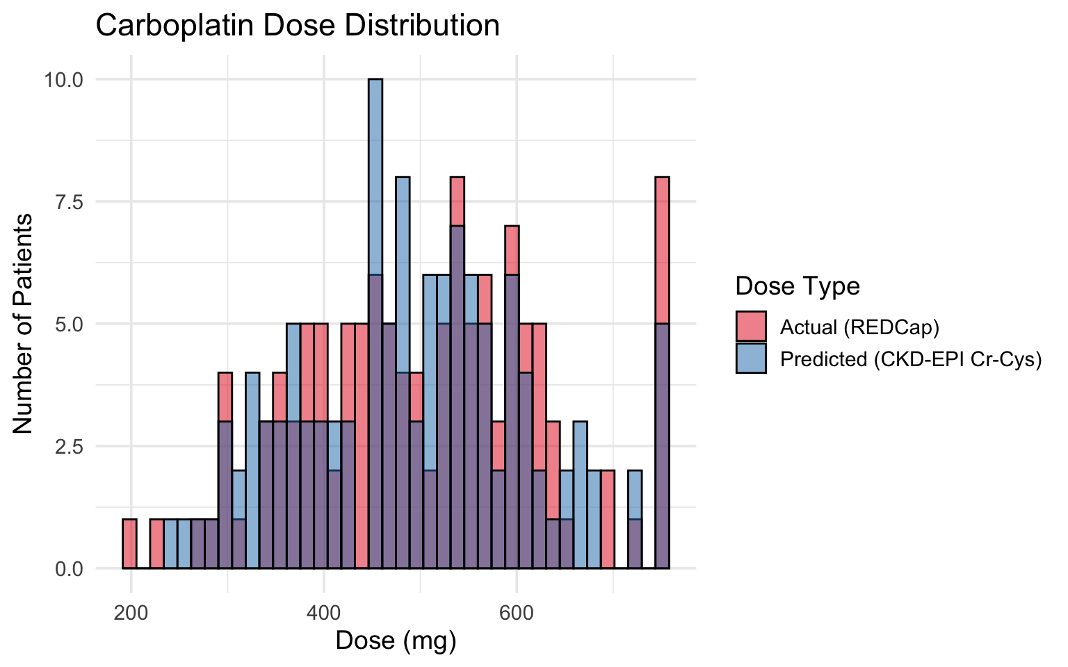
2.1 Actual vs Predicted Dose

Code
dose_long <- dat %>%
  select(record_id, carbo_dose_redcap, carbo_dose_cre_cys) %>%
  pivot_longer(
    cols = c(carbo_dose_redcap, carbo_dose_cre_cys),
    names_to = "dose_type", values_to = "dose_mg"
  ) %>%
  filter(!is.na(dose_mg)) %>%
  mutate(dose_type = case_match(dose_type,
    "carbo_dose_redcap"  ~ "Actual (REDCap)",
    "carbo_dose_cre_cys" ~ "Predicted (CKD-EPI Cr-Cys)"
  ))

ggplot(dose_long, aes(x = dose_mg, fill = dose_type)) +
  geom_histogram(alpha = 0.5, bins = 40, position = "identity", color = "black") +
  scale_fill_manual(values = c("Actual (REDCap)" = "#E31A1C",
                                "Predicted (CKD-EPI Cr-Cys)" = "#1F78B4")) +
  labs(title = "Carboplatin Dose Distribution",
       x = "Dose (mg)", y = "Number of Patients", fill = "Dose Type") +
  theme_minimal(base_size = 14) -> p
.save_plot_pptx(p)
p

2.2 Signed Dose Discrepancy Distribution

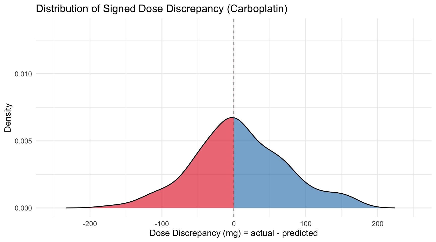
Smooth kernel density estimate of the signed dose discrepancy (actual − predicted, CKD-EPI Cr-Cys). The area under the curve is shaded by sign — negative (under-dosed region) on one side, positive on the other.

Code
dose_vals <- dat %>%
  filter(!is.na(dose_discrepancy)) %>%
  pull(dose_discrepancy)

dens <- density(dose_vals, n = 512)
y_at_zero <- approx(dens$x, dens$y, xout = 0)$y

dens_df <- tibble(x = dens$x, y = dens$y) %>%
  bind_rows(tibble(x = 0, y = y_at_zero)) %>%
  arrange(x)

neg_part <- dens_df %>% filter(x <= 0) %>% mutate(side = "neg")
pos_part <- dens_df %>% filter(x >= 0) %>% mutate(side = "pos")
plot_df  <- bind_rows(neg_part, pos_part)

ggplot() +
  geom_area(data = plot_df, aes(x = x, y = y, fill = side), alpha = 0.6) +
  geom_line(data = dens_df, aes(x = x, y = y), linewidth = 0.6, color = "black") +
  geom_vline(xintercept = 0, linetype = "dashed", color = "grey40") +
  scale_fill_manual(values = c(neg = "#E31A1C", pos = "#1F78B4"),
                    guide = "none") +
  coord_cartesian(xlim = c(-250, 250)) +
  labs(title = "Distribution of Signed Dose Discrepancy (Carboplatin)",
       x = "Dose Discrepancy (mg) = actual - predicted",
       y = "Density") +
  theme_minimal(base_size = 13) -> p
.save_plot_pptx(p)
p

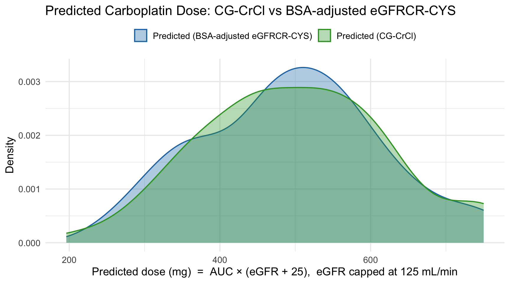
2.3 Predicted Dose: CG-CrCl vs BSA-adjusted eGFRCR-CYS

Overlay kernel density of the predicted carboplatin dose (Calvert formula, AUC × (eGFR + 25), eGFR capped at 125 mL/min) computed two ways: using Cockcroft-Gault creatinine clearance vs using the BSA-adjusted CKD-EPI Cr-Cys equation. Shows how the two kidney-function estimators would translate into different dose recommendations across the carboplatin cohort.

Code
dose_pred_long <- dat %>%
  mutate(carbo_dose_cg = carbo_AUC * (cockcroft_cap125 + 25)) %>%
  select(record_id, carbo_dose_cg, carbo_dose_cre_cys) %>%
  pivot_longer(
    cols = c(carbo_dose_cg, carbo_dose_cre_cys),
    names_to = "predictor", values_to = "dose_mg"
  ) %>%
  filter(!is.na(dose_mg)) %>%
  mutate(predictor = case_match(predictor,
    "carbo_dose_cg"      ~ "Predicted (CG-CrCl)",
    "carbo_dose_cre_cys" ~ "Predicted (BSA-adjusted eGFRCR-CYS)"
  ))

ggplot(dose_pred_long, aes(x = dose_mg, fill = predictor, color = predictor)) +
  geom_density(alpha = 0.35, linewidth = 0.7) +
  scale_fill_manual(values = c("Predicted (CG-CrCl)" = "#33A02C",
                                "Predicted (BSA-adjusted eGFRCR-CYS)" = "#1F78B4")) +
  scale_color_manual(values = c("Predicted (CG-CrCl)" = "#33A02C",
                                 "Predicted (BSA-adjusted eGFRCR-CYS)" = "#1F78B4")) +
  labs(title = "Predicted Carboplatin Dose: CG-CrCl vs BSA-adjusted eGFRCR-CYS",
       x = "Predicted dose (mg)  =  AUC × (eGFR + 25),  eGFR capped at 125 mL/min",
       y = "Density",
       fill = NULL, color = NULL) +
  theme_minimal(base_size = 14) +
  theme(legend.position = "top") -> p
.save_plot_pptx(p)
p

3 Table 1: Baseline Characteristics (Carboplatin Only)

Code
dat %>%
  dplyr::select(
    age, age_cat, sex, race, ethnicity, tumor_stage, cancer_type_cat_7,
    carbo_AUC, carbo_AUC_cat,
    ici, Bevacizumab, Paclitaxel, Pemetrexed, Doxorubicin, Etoposide,
    Gemcitabine, Pertuzumab, Trastuzumab, Docetaxel, other_chemo, Administered_alone,
    hiv_rpdr, thyroid, smoking, steroids,
    cci, score, ecog_score, bmi, bmi_cat,
    pre_HGB_45days, pre_PLT_45days, pre_ALB_45days,
    baseline_cys_c, baseline_cre, cr_cys,
    baseline_cre_egfr, baseline_cys_c_egfr,
    ckd_epi_gfr_cre_cys, ckd_stage_crcys, ckd_epi_gfr_cre_cys_unindex,
    cockcroft, egfr_ratio
  ) %>%
  tbl_summary(
    statistic = list(age ~ "{median} ({p25}, {p75})"),
    label = list(
      ckd_epi_gfr_cre_cys         ~ "eGFR CKD-EPI Cr-Cys, indexed (mL/min/1.73 m²)",
      ckd_stage_crcys             ~ "CKD stage (KDIGO G-stage, from indexed eGFR CKD-EPI Cr-Cys 2021)",
      ckd_epi_gfr_cre_cys_unindex ~ "BSA-adjusted eGFR CKD-EPI Cr-Cys (mL/min)",
      cockcroft                   ~ "Cockcroft-Gault CrCl (mL/min)",
      egfr_ratio                  ~ "eGFR ratio: CKD-EPI Cr-Cys / CG"
    )
  )
Characteristic N = 1211
age 70 (63, 76)
age_cat
    <=65 34 (28%)
    66-80 79 (65%)
    >80 8 (6.6%)
sex
    Female 61 (50%)
    Male 60 (50%)
race
    White 105 (87%)
    Black 2 (1.7%)
    Asian 7 (5.8%)
    Other 2 (1.7%)
    Unknown 5 (4.1%)
ethnicity
    Non-Hispanic 111 (92%)
    Hispanic 4 (3.3%)
    Unknown 6 (5.0%)
tumor_stage
    Local/Early 6 (5.0%)
    Advanced/Metastatic 115 (95%)
cancer_type_cat_7
    Thoracic 121 (100%)
    Breast 0 (0%)
    GI 0 (0%)
    GU 0 (0%)
    GYN 0 (0%)
    HEENT 0 (0%)
    Other 0 (0%)
carbo_AUC
    3 5 (4.1%)
    4 24 (20%)
    5 92 (76%)
carbo_AUC_cat
    <3 0 (0%)
    >=3 121 (100%)
ici 58 (48%)
Bevacizumab
    0 121 (100%)
Paclitaxel
    0 121 (100%)
Pemetrexed
    1 121 (100%)
Doxorubicin
    0 121 (100%)
Etoposide
    0 121 (100%)
Gemcitabine
    0 121 (100%)
Pertuzumab
    0 121 (100%)
Trastuzumab
    0 121 (100%)
Docetaxel
    0 121 (100%)
other_chemo
    0 121 (100%)
Administered_alone
    0 121 (100%)
hiv_rpdr 3 (2.5%)
thyroid 20 (17%)
smoking 76 (63%)
steroids 119 (98%)
cci
    moderate 2 (1.7%)
    severe 119 (98%)
score 10.00 (8.00, 12.00)
ecog_score
    0 28 (23%)
    1 77 (64%)
    2 13 (11%)
    3 3 (2.5%)
bmi 26.1 (23.4, 29.5)
bmi_cat
    Underweight (<18.5) 4 (3.3%)
    Normal (18.5-25) 42 (35%)
    Overweight (25-30) 49 (40%)
    Obese (>=30) 26 (21%)
pre_HGB_45days 12.90 (11.70, 13.90)
pre_PLT_45days 264 (214, 344)
pre_ALB_45days 4.20 (4.00, 4.40)
baseline_cys_c 1.11 (0.93, 1.30)
baseline_cre 0.83 (0.71, 0.99)
cr_cys 0.73 (0.64, 0.85)
baseline_cre_egfr 88 (74, 96)
baseline_cys_c_egfr 63 (52, 76)
eGFR CKD-EPI Cr-Cys, indexed (mL/min/1.73 m²) 74 (65, 89)
CKD stage (KDIGO G-stage, from indexed eGFR CKD-EPI Cr-Cys 2021)
    G1 (>=90) 27 (22%)
    G2 (60-89) 71 (59%)
    G3a (45-59) 19 (16%)
    G3b (30-44) 3 (2.5%)
    G4 (15-29) 1 (0.8%)
    G5 (<15) 0 (0%)
BSA-adjusted eGFR CKD-EPI Cr-Cys (mL/min) 78 (66, 94)
Cockcroft-Gault CrCl (mL/min) 79 (64, 96)
eGFR ratio: CKD-EPI Cr-Cys / CG 0.99 (0.86, 1.10)
1 Median (Q1, Q3); n (%)

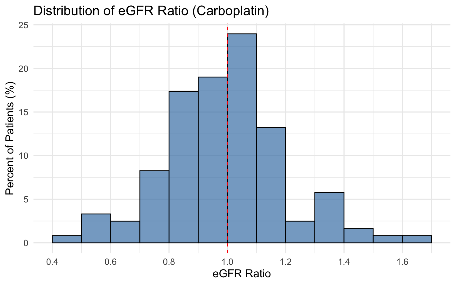
4 eGFR Ratio Distribution (Carboplatin)

Code
ratio_hist <- dat %>% filter(!is.na(egfr_ratio))

ggplot(ratio_hist, aes(x = egfr_ratio)) +
  geom_histogram(aes(y = after_stat(count) / sum(after_stat(count)) * 100),
                 binwidth = 0.1, boundary = 0,
                 fill = "steelblue", color = "black", alpha = 0.7) +
  geom_vline(xintercept = 1, linetype = "dashed", color = "red") +
  labs(title = "Distribution of eGFR Ratio (Carboplatin)",
       x = "eGFR Ratio",
       y = "Percent of Patients (%)") +
  scale_x_continuous(breaks = seq(0, 3, 0.2)) +
  theme_minimal(base_size = 14) -> p
.save_plot_pptx(p)
p

Event Counts by Outcome (Diagnostic)

For each outcome the table below shows the cohort N, events (status = 1 within 90 days), competing deaths (status = 2; not applicable to 90-day death which is modelled by Cox PH), censored, event rate, and events-per-variable (EPV) using the 5-variable base adjuster set for this cohort (age, sex, ecog_score (ECOG performance status, numeric 0–5), ici, cockcroft (creatinine clearance)). Following the Jiaxuan-paper methodology, anemia models additionally adjust for pre_HGB_45days (baseline hemoglobin within 45 days), thrombocytopenia models additionally adjust for pre_PLT_45days (baseline platelets within 45 days), and the composite Grade 2 / Grade 3 cytopenia models (which combine anemia, thrombocytopenia, and AKI events) adjust for both pre_HGB_45days and pre_PLT_45days — so anemia / throm outcomes carry 6 adjusters and the composites carry 7. Read the EPV column against the per-outcome adjuster count, not the base 5. As a rule of thumb, Fine-Gray fits need ≥ 5 × adj events to be stable; < 2 × adj almost always produces a singular design matrix, which is why the helper functions in this file fall back to a “Model could not be fit” placeholder where you see one.

Code
.outcomes_tbl <- function(dat, cohort_label, n_adj = 5) {
  sumrow <- function(label, status_var, is_cox = FALSE) {
    s <- suppressWarnings(as.integer(as.character(dat[[status_var]])))
    n_total     <- sum(!is.na(s))
    n_event     <- sum(s == 1, na.rm = TRUE)
    n_compdeath <- if (is_cox) NA_integer_ else sum(s == 2, na.rm = TRUE)
    n_cens      <- sum(s == 0, na.rm = TRUE)
    epv         <- if (n_total > 0) n_event / n_adj else NA_real_
    fit_likely  <- if (is.na(epv))                "—"
                   else if (n_event >= 5 * n_adj) "✓ likely OK"
                   else if (n_event >= 2 * n_adj) "marginal"
                   else                           "✗ singular likely"
    tibble::tibble(
      Outcome            = label,
      N                  = n_total,
      Events             = n_event,
      `Competing deaths` = n_compdeath,
      Censored           = n_cens,
      `Event rate`       = if (n_total > 0) sprintf("%.1f%%", 100 * n_event / n_total) else "—",
      EPV                = if (!is.na(epv)) sprintf("%.1f", epv) else "—",
      `Fit reliable?`    = fit_likely
    )
  }
  dplyr::bind_rows(
    sumrow("Anemia Grade 2",                   "cmp_status_anemia_2"),
    sumrow("Anemia Grade 3",                   "cmp_status_anemia_3"),
    sumrow("Thrombocytopenia Grade 2",         "cmp_status_throm_2"),
    sumrow("Thrombocytopenia Grade 3",         "cmp_status_throm_3"),
    sumrow("AKI Grade 2",                      "cmp_status_aki_2"),
    sumrow("AKI (KDIGO)",                      "cmp_status_aki_kdigo"),
    sumrow("Composite Grade 2 AEs",            "cmp_status_grade_2_aes"),
    sumrow("Composite Grade 3 AEs",            "cmp_status_grade_3_aes"),
    sumrow("Overall Hospitalization",          "cmp_status_any_hosp"),
    sumrow("Platinum-Related Hospitalization", "cmp_status_side_effect"),
    sumrow("90-Day Death (Cox PH)",            "death_90", is_cox = TRUE)
  )
}

knitr::kable(
  .outcomes_tbl(dat, "carboplatin cohort"),
  align = c("l","r","r","r","r","r","r","l"),
  caption = sprintf(
    "Event counts for the **carboplatin cohort** (N = %d). EPV uses 5 base adjusters (age, sex, ecog_score, ici, cockcroft); anemia / thrombocytopenia models add pre_HGB_45days / pre_PLT_45days for 6 total.",
    nrow(dat)
  )
)
Event counts for the carboplatin cohort (N = 121). EPV uses 5 base adjusters (age, sex, ecog_score, ici, cockcroft); anemia / thrombocytopenia models add pre_HGB_45days / pre_PLT_45days for 6 total.
Outcome N Events Competing deaths Censored Event rate EPV Fit reliable?
Anemia Grade 2 121 42 5 74 34.7% 8.4 ✓ likely OK
Anemia Grade 3 121 14 8 99 11.6% 2.8 marginal
Thrombocytopenia Grade 2 121 16 7 98 13.2% 3.2 marginal
Thrombocytopenia Grade 3 121 10 8 103 8.3% 2.0 marginal
AKI Grade 2 121 8 9 104 6.6% 1.6 ✗ singular likely
AKI (KDIGO) 121 11 9 101 9.1% 2.2 marginal
Composite Grade 2 AEs 121 47 5 69 38.8% 9.4 ✓ likely OK
Composite Grade 3 AEs 121 16 8 97 13.2% 3.2 marginal
Overall Hospitalization 121 29 4 88 24.0% 5.8 ✓ likely OK
Platinum-Related Hospitalization 121 21 5 95 17.4% 4.2 marginal
90-Day Death (Cox PH) 121 10 NA 111 8.3% 2.0 marginal

5 Fine-Gray Models — eGFR Ratio (Carboplatin)

Each table below shows univariable (one variable at a time) and multivariable Fine-Gray subdistribution hazard ratios side-by-side. A Word version of every table is saved during render — click any link below to download:

Code
.adj_set <- function(pre_labs, egfr_adj) {
  # Sherley sub-cohort (N=169) adjuster set:
  #   - 5 base confounders: age, sex, ecog_score, ici, cockcroft
  #   - + pre_labs when supplied — anemia models pass "pre_HGB_45days"
  #     and thrombocytopenia models pass "pre_PLT_45days" to match the
  #     Jiaxuan-paper methodology (baseline hemoglobin / platelets).
  # The egfr_adj argument is accepted for backward compatibility but
  # cockcroft is already in the base set so it is effectively ignored.
  adj <- c("age", "sex", "ecog_score", "ici", "cockcroft")
  if (!is.null(pre_labs)) adj <- c(adj, pre_labs)
  adj
}

# fg_model: returns univariable + multivariable merged Fine-Gray table.
# If docx_name is supplied, also saves the table as a .docx in docx_dir.
fg_model <- function(time_var, status_var, pred_var, pre_labs = NULL,
                     egfr_adj = c("none", "cockcroft", "ckd_epi"),
                     docx_name = NULL) {
  egfr_adj <- match.arg(egfr_adj)
  adj <- .adj_set(pre_labs, egfr_adj)
  all_vars <- c(pred_var, adj)

  fmla_mv <- as.formula(paste0(
    "Surv(", time_var, ", ", status_var, ") ~ ",
    paste(all_vars, collapse = " + ")
  ))
  tbl_mv <- tryCatch(
    tidycmprsk::crr(fmla_mv, failcode = 1, data = dat) %>%
      tbl_regression(exp = TRUE,
                     pvalue_fun = function(x) style_pvalue(x, digits = 3)) %>%
      add_n(),
    error = function(e) NULL
  )

  y_call <- str2lang(sprintf("Surv(%s, %s)", time_var, status_var))
  tbl_uv <- tryCatch(
    rlang::inject(
      tbl_uvregression(
        data = dat,
        method = tidycmprsk::crr,
        y = !!y_call,
        include = dplyr::all_of(all_vars),
        exponentiate = TRUE,
        pvalue_fun = function(x) style_pvalue(x, digits = 3),
        method.args = list(failcode = 1)
      )
    ),
    error = function(e) NULL
  )

  if (is.null(tbl_uv) && is.null(tbl_mv)) {
    return(knitr::asis_output(
      "> *Model could not be fit — Fine-Gray design matrix is singular (insufficient events or collinear covariates for this sub-cohort).*"
    ))
  }

  out <- if (is.null(tbl_mv)) {
    tbl_uv
  } else if (is.null(tbl_uv)) {
    tbl_mv
  } else {
    tbl_merge(
      tbls = list(tbl_uv, tbl_mv),
      tab_spanner = c("**Univariable**", "**Multivariable**")
    )
  }

  if (!is.null(docx_name)) save_tbl_docx(out, docx_name)
  out
}

cox_model <- function(time_var, status_var, pred_var, pre_labs = NULL,
                      egfr_adj = c("none", "cockcroft", "ckd_epi"),
                      docx_name = NULL) {
  egfr_adj <- match.arg(egfr_adj)
  adj <- .adj_set(pre_labs, egfr_adj)
  all_vars <- c(pred_var, adj)

  fmla_mv <- as.formula(paste0(
    "Surv(", time_var, ", ", status_var, ") ~ ",
    paste(all_vars, collapse = " + ")
  ))
  tbl_mv <- survival::coxph(fmla_mv, data = dat) %>%
    tbl_regression(exp = TRUE,
                   pvalue_fun = function(x) style_pvalue(x, digits = 3)) %>%
    add_n()

  y_call <- str2lang(sprintf("Surv(%s, %s)", time_var, status_var))
  tbl_uv <- rlang::inject(
    tbl_uvregression(
      data = dat,
      method = survival::coxph,
      y = !!y_call,
      include = dplyr::all_of(all_vars),
      exponentiate = TRUE,
      pvalue_fun = function(x) style_pvalue(x, digits = 3)
    )
  )

  out <- tbl_merge(
    tbls = list(tbl_uv, tbl_mv),
    tab_spanner = c("**Univariable**", "**Multivariable**")
  )

  if (!is.null(docx_name)) save_tbl_docx(out, docx_name)
  out
}

4.1 Anemia Grade 2

Code
fg_model("cmp_time_anemia_2", "cmp_status_anemia_2", "egfr_ratio_per10", "pre_HGB_45days", "cockcroft", docx_name = "sec5_anemia_2")
Characteristic
Univariable
Multivariable
N HR1 95% CI1 p-value N HR1 95% CI1 p-value
egfr_ratio_per10 121 1.29 1.11, 1.50 0.001 121 1.29 1.01, 1.65 0.043
age 121 1.00 0.97, 1.03 0.880 121 1.01 0.97, 1.05 0.570
sex 121


121


    Female
— —

— —
    Male
1.04 0.58, 1.89 0.890
1.67 0.89, 3.17 0.110
ecog_score 121 1.46 0.97, 2.19 0.070 121 1.18 0.65, 2.13 0.590
ici 121 0.87 0.47, 1.59 0.640 121 1.11 0.59, 2.07 0.750
cockcroft 121 1.00 0.99, 1.01 0.840 121 0.99 0.98, 1.01 0.260
pre_HGB_45days 121 0.51 0.42, 0.63 <0.001 121 0.54 0.43, 0.67 <0.001
1 HR = Hazard Ratio, CI = Confidence Interval

4.2 Anemia Grade 3

Code
fg_model("cmp_time_anemia_3", "cmp_status_anemia_3", "egfr_ratio_per10", "pre_HGB_45days", "cockcroft", docx_name = "sec5_anemia_3")
Characteristic
Univariable
Multivariable
N HR1 95% CI1 p-value N HR1 95% CI1 p-value
egfr_ratio_per10 121 1.44 1.13, 1.85 0.004 121 1.33 0.88, 2.03 0.180
age 121 1.02 0.96, 1.07 0.570 121 1.03 0.96, 1.11 0.410
sex 121


121


    Female
— —

— —
    Male
1.95 0.66, 5.71 0.220
2.19 0.63, 7.66 0.220
ecog_score 121 1.59 0.94, 2.70 0.086 121 1.74 0.54, 5.62 0.360
ici 121 1.56 0.55, 4.39 0.400 121 1.54 0.46, 5.17 0.490
cockcroft 121 1.01 0.99, 1.02 0.570 121 0.99 0.97, 1.01 0.420
pre_HGB_45days 121 0.44 0.31, 0.61 <0.001 121 0.47 0.29, 0.76 0.002
1 HR = Hazard Ratio, CI = Confidence Interval

4.3 Thrombocytopenia Grade 2

Code
fg_model("cmp_time_throm_2", "cmp_status_throm_2", "egfr_ratio_per10", "pre_PLT_45days", "cockcroft", docx_name = "sec5_throm_2")
Characteristic
Univariable
Multivariable
N HR1 95% CI1 p-value N HR1 95% CI1 p-value
egfr_ratio_per10 121 1.56 1.22, 1.99 <0.001 121 1.65 1.08, 2.53 0.021
age 121 0.98 0.93, 1.03 0.350 121 1.00 0.93, 1.07 0.920
sex 121


121


    Female
— —

— —
    Male
1.04 0.40, 2.74 0.930
1.18 0.47, 2.99 0.730
ecog_score 121 1.93 1.23, 3.03 0.004 121 1.06 0.48, 2.34 0.890
ici 121 1.10 0.42, 2.89 0.850 121 1.35 0.40, 4.54 0.630
cockcroft 121 1.01 1.00, 1.03 0.095 121 1.0 0.98, 1.01 0.580
pre_PLT_45days 121 1.00 0.99, 1.00 0.670 121 1.00 0.99, 1.00 0.570
1 HR = Hazard Ratio, CI = Confidence Interval

4.4 Thrombocytopenia Grade 3

Code
fg_model("cmp_time_throm_3", "cmp_status_throm_3", "egfr_ratio_per10", "pre_PLT_45days", "cockcroft", docx_name = "sec5_throm_3")
Characteristic
Univariable
Multivariable
N HR1 95% CI1 p-value N HR1 95% CI1 p-value
egfr_ratio_per10 121 1.81 1.32, 2.48 <0.001 121 2.47 1.32, 4.60 0.005
age 121 1.00 0.94, 1.06 0.980 121 1.04 0.94, 1.16 0.400
sex 121


121


    Female
— —

— —
    Male
2.53 0.67, 9.54 0.170
2.35 0.57, 9.64 0.240
ecog_score 121 1.75 1.06, 2.88 0.029 121 0.55 0.19, 1.62 0.280
ici 121 1.69 0.48, 5.89 0.410 121 1.07 0.26, 4.48 0.920
cockcroft 121 1.02 1.00, 1.04 0.027 121 1.00 0.98, 1.02 0.900
pre_PLT_45days 121 1.00 0.99, 1.01 0.900 121 1.00 1.00, 1.01 0.960
1 HR = Hazard Ratio, CI = Confidence Interval

4.5 AKI Grade 2

Code
fg_model("cmp_time_aki_2", "cmp_status_aki_2", "egfr_ratio_per10", egfr_adj = "cockcroft", docx_name = "sec5_aki_2")
Characteristic
Univariable
Multivariable
N HR1 95% CI1 p-value N HR1 95% CI1 p-value
egfr_ratio_per10 121 1.40 0.97, 2.03 0.074 121 1.18 0.79, 1.75 0.420
age 121 1.00 0.95, 1.06 0.890 121 1.02 0.91, 1.14 0.780
sex 121


121


    Female
— —

— —
    Male
1.74 0.42, 7.18 0.440
1.70 0.31, 9.35 0.540
ecog_score 121 2.33 1.29, 4.22 0.005 121 2.26 0.74, 6.90 0.150
ici 121 1.88 0.46, 7.71 0.380 121 2.20 0.44, 10.9 0.330
cockcroft 121 1.01 1.00, 1.03 0.062 121 1.00 0.99, 1.02 0.760
1 HR = Hazard Ratio, CI = Confidence Interval

4.6 AKI (KDIGO)

Code
fg_model("cmp_time_aki_kdigo", "cmp_status_aki_kdigo", "egfr_ratio_per10", egfr_adj = "cockcroft", docx_name = "sec5_aki_kdigo")
Characteristic
Univariable
Multivariable
N HR1 95% CI1 p-value N HR1 95% CI1 p-value
egfr_ratio_per10 121 1.38 1.05, 1.82 0.023 121 1.42 0.92, 2.20 0.120
age 121 1.02 0.97, 1.06 0.540 121 1.04 0.94, 1.14 0.430
sex 121


121


    Female
— —

— —
    Male
1.24 0.38, 4.00 0.720
1.04 0.23, 4.64 0.960
ecog_score 121 1.69 0.90, 3.18 0.100 121 1.17 0.35, 3.96 0.800
ici 121 1.98 0.59, 6.68 0.270 121 1.91 0.55, 6.68 0.310
cockcroft 121 1.01 0.99, 1.02 0.220 121 1.00 0.98, 1.02 0.990
1 HR = Hazard Ratio, CI = Confidence Interval

4.7 Composite Grade 2 AEs

Code
fg_model("cmp_time_grade_2_aes", "cmp_status_grade_2_aes", "egfr_ratio_per10", pre_labs = c("pre_HGB_45days", "pre_PLT_45days"), egfr_adj = "cockcroft", docx_name = "sec5_grade_2_aes")
Characteristic
Univariable
Multivariable
N HR1 95% CI1 p-value N HR1 95% CI1 p-value
egfr_ratio_per10 121 1.25 1.09, 1.44 0.002 121 1.17 0.94, 1.45 0.150
age 121 0.99 0.96, 1.02 0.600 121 1.00 0.96, 1.04 0.990
sex 121


121


    Female
— —

— —
    Male
1.11 0.63, 1.95 0.710
1.71 0.94, 3.12 0.079
ecog_score 121 1.51 1.03, 2.21 0.035 121 1.31 0.78, 2.19 0.300
ici 121 0.83 0.47, 1.48 0.530 121 1.11 0.60, 2.07 0.730
cockcroft 121 1.00 0.99, 1.01 0.570 121 1.00 0.98, 1.01 0.510
pre_HGB_45days 121 0.58 0.49, 0.69 <0.001 121 0.57 0.45, 0.72 <0.001
pre_PLT_45days 121 1.00 1.00, 1.00 0.470 121 1.00 1.00, 1.00 0.390
1 HR = Hazard Ratio, CI = Confidence Interval

4.8 Composite Grade 3 AEs

Code
fg_model("cmp_time_grade_3_aes", "cmp_status_grade_3_aes", "egfr_ratio_per10", pre_labs = c("pre_HGB_45days", "pre_PLT_45days"), egfr_adj = "cockcroft", docx_name = "sec5_grade_3_aes")
Characteristic
Univariable
Multivariable
N HR1 95% CI1 p-value N HR1 95% CI1 p-value
egfr_ratio_per10 121 1.53 1.21, 1.93 <0.001 121 1.48 0.91, 2.40 0.110
age 121 1.00 0.95, 1.05 0.940 121 1.02 0.94, 1.11 0.590
sex 121


121


    Female
— —

— —
    Male
1.83 0.68, 4.93 0.230
2.01 0.50, 8.11 0.330
ecog_score 121 1.72 1.04, 2.82 0.033 121 1.24 0.46, 3.39 0.670
ici 121 1.15 0.44, 3.02 0.780 121 0.99 0.31, 3.13 0.990
cockcroft 121 1.01 1.00, 1.03 0.110 121 1.00 0.98, 1.02 0.810
pre_HGB_45days 121 0.48 0.35, 0.64 <0.001 121 0.56 0.39, 0.82 0.003
pre_PLT_45days 121 1.01 1.00, 1.01 0.001 121 1.00 1.00, 1.01 0.610
1 HR = Hazard Ratio, CI = Confidence Interval

4.9 Overall Hospitalization

Code
fg_model("cmp_time_any_hosp", "cmp_status_any_hosp", "egfr_ratio_per10", egfr_adj = "cockcroft", docx_name = "sec5_any_hosp")
Characteristic
Univariable
Multivariable
N HR1 95% CI1 p-value N HR1 95% CI1 p-value
egfr_ratio_per10 121 1.29 1.07, 1.54 0.007 121 1.48 1.17, 1.85 <0.001
age 121 1.02 0.97, 1.07 0.540 121 1.04 0.98, 1.11 0.240
sex 121


121


    Female
— —

— —
    Male
1.15 0.56, 2.36 0.700
1.30 0.63, 2.66 0.470
ecog_score 121 1.45 0.89, 2.36 0.130 121 1.02 0.54, 1.93 0.960
ici 121 0.91 0.44, 1.88 0.800 121 0.86 0.37, 1.99 0.730
cockcroft 121 1.00 0.99, 1.01 0.680 121 0.99 0.98, 1.01 0.300
1 HR = Hazard Ratio, CI = Confidence Interval

4.11 90-Day Death (Cox PH)

Code
cox_model("time_to_death_90", "death_90", "egfr_ratio_per10", egfr_adj = "cockcroft", docx_name = "sec5_death_90")
Characteristic
Univariable
Multivariable
N HR1 95% CI1 p-value N HR1 95% CI1 p-value
egfr_ratio_per10 121 1.63 1.16, 2.29 0.005 121 1.55 1.06, 2.29 0.025
age 121 1.02 0.95, 1.10 0.539 121 1.05 0.95, 1.15 0.329
sex 121


121


    Female
— —

— —
    Male
1.60 0.45, 5.66 0.468
3.13 0.68, 14.5 0.145
ecog_score 121 3.85 1.91, 7.76 <0.001 121 3.94 1.49, 10.4 0.006
ici 121 0.73 0.21, 2.60 0.632 121 1.01 0.22, 4.62 0.989
cockcroft 121 1.01 0.99, 1.03 0.357 121 0.99 0.97, 1.01 0.294
1 HR = Hazard Ratio, CI = Confidence Interval

6 Cause-Specific Hazard Models — eGFR Ratio (Carboplatin)

Code
csh_model <- function(time_var, status_var, pred_var, pre_labs = NULL) {
  adj <- c("age", "sex", "ecog_score", "ici", "cockcroft")
  if (!is.null(pre_labs)) adj <- c(adj, pre_labs)
  d <- dat
  d$csh_status <- ifelse(d[[status_var]] == 1, 1L, 0L)
  fmla <- as.formula(paste0(
    "Surv(", time_var, ", csh_status) ~ ",
    paste(c(pred_var, adj), collapse = " + ")
  ))
  tryCatch(
    survival::coxph(fmla, data = d) %>%
      tbl_regression(exp = TRUE,
                     pvalue_fun = function(x) style_pvalue(x, digits = 3)) %>%
      add_n(),
    error = function(e) .tbl_failed()
  )
}

5.1 Anemia Grade 2

Code
csh_model("cmp_time_anemia_2", "cmp_status_anemia_2", "egfr_ratio_per10", "pre_HGB_45days")
Characteristic N HR1 95% CI1 p-value
egfr_ratio_per10 121 1.35 1.07, 1.70 0.011
age 121 1.02 0.98, 1.07 0.267
sex 121


    Female
— —
    Male
1.53 0.79, 2.95 0.203
ecog_score 121 1.47 0.87, 2.48 0.154
ici 121 0.93 0.49, 1.76 0.818
cockcroft 121 0.99 0.98, 1.00 0.055
pre_HGB_45days 121 0.48 0.37, 0.62 <0.001
1 HR = Hazard Ratio, CI = Confidence Interval

5.2 Anemia Grade 3

Code
csh_model("cmp_time_anemia_3", "cmp_status_anemia_3", "egfr_ratio_per10", "pre_HGB_45days")
Characteristic N HR1 95% CI1 p-value
egfr_ratio_per10 121 1.35 0.90, 2.01 0.148
age 121 1.05 0.96, 1.14 0.274
sex 121


    Female
— —
    Male
2.24 0.59, 8.46 0.236
ecog_score 121 2.32 0.87, 6.21 0.095
ici 121 1.22 0.36, 4.06 0.749
cockcroft 121 0.99 0.97, 1.01 0.368
pre_HGB_45days 121 0.41 0.25, 0.66 <0.001
1 HR = Hazard Ratio, CI = Confidence Interval

5.3 Thrombocytopenia Grade 2

Code
csh_model("cmp_time_throm_2", "cmp_status_throm_2", "egfr_ratio_per10", "pre_PLT_45days")
Characteristic N HR1 95% CI1 p-value
egfr_ratio_per10 121 1.71 1.13, 2.58 0.011
age 121 1.00 0.93, 1.06 0.944
sex 121


    Female
— —
    Male
1.25 0.42, 3.68 0.692
ecog_score 121 1.14 0.46, 2.82 0.783
ici 121 1.39 0.44, 4.40 0.574
cockcroft 121 0.99 0.98, 1.01 0.459
pre_PLT_45days 121 1.00 0.99, 1.00 0.493
1 HR = Hazard Ratio, CI = Confidence Interval

5.4 Thrombocytopenia Grade 3

Code
csh_model("cmp_time_throm_3", "cmp_status_throm_3", "egfr_ratio_per10", "pre_PLT_45days")
Characteristic N HR1 95% CI1 p-value
egfr_ratio_per10 121 2.58 1.43, 4.66 0.002
age 121 1.04 0.95, 1.15 0.395
sex 121


    Female
— —
    Male
2.73 0.57, 13.0 0.207
ecog_score 121 0.62 0.19, 2.05 0.436
ici 121 1.13 0.26, 4.94 0.872
cockcroft 121 1.00 0.98, 1.02 0.836
pre_PLT_45days 121 1.00 0.99, 1.01 0.981
1 HR = Hazard Ratio, CI = Confidence Interval

5.5 AKI Grade 2

Code
csh_model("cmp_time_aki_2", "cmp_status_aki_2", "egfr_ratio_per10")
Characteristic N HR1 95% CI1 p-value
egfr_ratio_per10 121 1.21 0.75, 1.95 0.434
age 121 1.02 0.92, 1.12 0.759
sex 121


    Female
— —
    Male
1.82 0.39, 8.61 0.449
ecog_score 121 2.45 0.72, 8.37 0.152
ici 121 2.22 0.43, 11.4 0.339
cockcroft 121 1.00 0.98, 1.02 0.896
1 HR = Hazard Ratio, CI = Confidence Interval

5.6 AKI (KDIGO)

Code
csh_model("cmp_time_aki_kdigo", "cmp_status_aki_kdigo", "egfr_ratio_per10")
Characteristic N HR1 95% CI1 p-value
egfr_ratio_per10 121 1.44 0.94, 2.20 0.096
age 121 1.04 0.95, 1.13 0.372
sex 121


    Female
— —
    Male
1.08 0.30, 3.88 0.912
ecog_score 121 1.25 0.40, 3.89 0.699
ici 121 1.86 0.48, 7.14 0.367
cockcroft 121 1.00 0.98, 1.02 0.955
1 HR = Hazard Ratio, CI = Confidence Interval

5.7 Composite Grade 2 AEs

Code
csh_model("cmp_time_grade_2_aes", "cmp_status_grade_2_aes", "egfr_ratio_per10", c("pre_HGB_45days", "pre_PLT_45days"))
Characteristic N HR1 95% CI1 p-value
egfr_ratio_per10 121 1.21 0.98, 1.50 0.070
age 121 1.01 0.97, 1.05 0.619
sex 121


    Female
— —
    Male
1.61 0.86, 3.01 0.133
ecog_score 121 1.52 0.95, 2.43 0.083
ici 121 1.04 0.55, 1.99 0.899
cockcroft 121 0.99 0.98, 1.00 0.229
pre_HGB_45days 121 0.50 0.39, 0.66 <0.001
pre_PLT_45days 121 1.00 0.99, 1.00 0.146
1 HR = Hazard Ratio, CI = Confidence Interval

5.8 Composite Grade 3 AEs

Code
csh_model("cmp_time_grade_3_aes", "cmp_status_grade_3_aes", "egfr_ratio_per10", c("pre_HGB_45days", "pre_PLT_45days"))
Characteristic N HR1 95% CI1 p-value
egfr_ratio_per10 121 1.49 0.96, 2.31 0.074
age 121 1.03 0.96, 1.10 0.424
sex 121


    Female
— —
    Male
2.30 0.64, 8.21 0.199
ecog_score 121 1.67 0.68, 4.15 0.266
ici 121 0.81 0.27, 2.47 0.712
cockcroft 121 1.00 0.98, 1.01 0.690
pre_HGB_45days 121 0.51 0.33, 0.80 0.003
pre_PLT_45days 121 1.00 1.00, 1.01 0.398
1 HR = Hazard Ratio, CI = Confidence Interval

5.9 Overall Hospitalization

Code
csh_model("cmp_time_any_hosp", "cmp_status_any_hosp", "egfr_ratio_per10")
Characteristic N HR1 95% CI1 p-value
egfr_ratio_per10 121 1.52 1.17, 1.98 0.002
age 121 1.04 0.99, 1.10 0.119
sex 121


    Female
— —
    Male
1.28 0.59, 2.76 0.534
ecog_score 121 1.06 0.55, 2.02 0.861
ici 121 0.84 0.38, 1.85 0.663
cockcroft 121 0.99 0.98, 1.01 0.235
1 HR = Hazard Ratio, CI = Confidence Interval

5.11 90-Day Death (Cox PH)

Code
cox_model("time_to_death_90", "death_90", "egfr_ratio_per10", egfr_adj = "cockcroft")
Characteristic
Univariable
Multivariable
N HR1 95% CI1 p-value N HR1 95% CI1 p-value
egfr_ratio_per10 121 1.63 1.16, 2.29 0.005 121 1.55 1.06, 2.29 0.025
age 121 1.02 0.95, 1.10 0.539 121 1.05 0.95, 1.15 0.329
sex 121


121


    Female
— —

— —
    Male
1.60 0.45, 5.66 0.468
3.13 0.68, 14.5 0.145
ecog_score 121 3.85 1.91, 7.76 <0.001 121 3.94 1.49, 10.4 0.006
ici 121 0.73 0.21, 2.60 0.632 121 1.01 0.22, 4.62 0.989
cockcroft 121 1.01 0.99, 1.03 0.357 121 0.99 0.97, 1.01 0.294
1 HR = Hazard Ratio, CI = Confidence Interval

7 Fine-Gray Models — Dose Discrepancy per 25 mg (Carboplatin)

7.1 Anemia Grade 2

Code
fg_model("cmp_time_anemia_2", "cmp_status_anemia_2", "dose_discrep_per25increase", "pre_HGB_45days", "cockcroft")
Characteristic
Univariable
Multivariable
N HR1 95% CI1 p-value N HR1 95% CI1 p-value
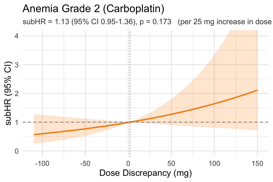
dose_discrep_per25increase 121 1.19 1.05, 1.35 0.005 121 1.13 0.95, 1.36 0.170
age 121 1.00 0.97, 1.03 0.880 121 1.01 0.97, 1.05 0.590
sex 121


121


    Female
— —

— —
    Male
1.04 0.58, 1.89 0.890
1.58 0.85, 2.95 0.150
ecog_score 121 1.46 0.97, 2.19 0.070 121 1.31 0.76, 2.27 0.340
ici 121 0.87 0.47, 1.59 0.640 121 1.14 0.60, 2.16 0.700
cockcroft 121 1.00 0.99, 1.01 0.840 121 1.00 0.98, 1.01 0.480
pre_HGB_45days 121 0.51 0.42, 0.63 <0.001 121 0.52 0.42, 0.64 <0.001
1 HR = Hazard Ratio, CI = Confidence Interval

7.2 Anemia Grade 3

Code
fg_model("cmp_time_anemia_3", "cmp_status_anemia_3", "dose_discrep_per25increase", "pre_HGB_45days", "cockcroft")
Characteristic
Univariable
Multivariable
N HR1 95% CI1 p-value N HR1 95% CI1 p-value
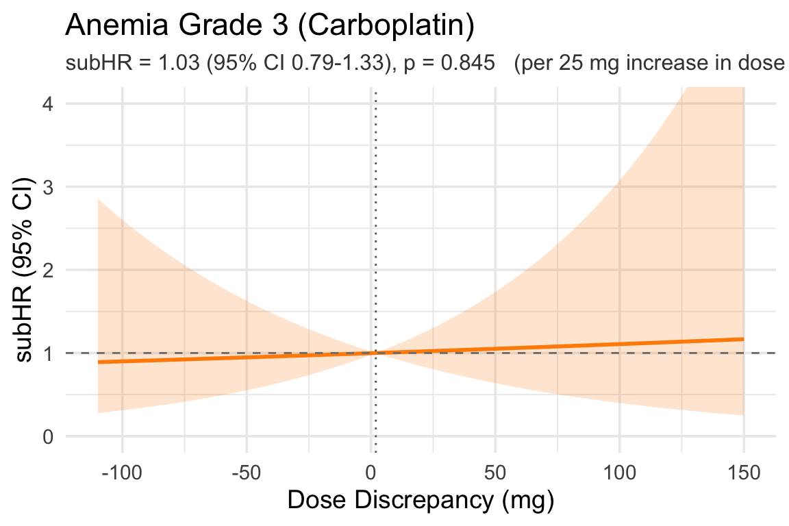
dose_discrep_per25increase 121 1.24 1.03, 1.49 0.023 121 1.03 0.79, 1.33 0.850
age 121 1.02 0.96, 1.07 0.570 121 1.03 0.95, 1.10 0.470
sex 121


121


    Female
— —

— —
    Male
1.95 0.66, 5.71 0.220
2.02 0.65, 6.24 0.220
ecog_score 121 1.59 0.94, 2.70 0.086 121 2.24 0.76, 6.58 0.140
ici 121 1.56 0.55, 4.39 0.400 121 1.62 0.51, 5.15 0.410
cockcroft 121 1.01 0.99, 1.02 0.570 121 1.00 0.97, 1.02 0.780
pre_HGB_45days 121 0.44 0.31, 0.61 <0.001 121 0.43 0.27, 0.69 <0.001
1 HR = Hazard Ratio, CI = Confidence Interval

7.3 Thrombocytopenia Grade 2

Code
fg_model("cmp_time_throm_2", "cmp_status_throm_2", "dose_discrep_per25increase", "pre_PLT_45days", "cockcroft")
Characteristic
Univariable
Multivariable
N HR1 95% CI1 p-value N HR1 95% CI1 p-value
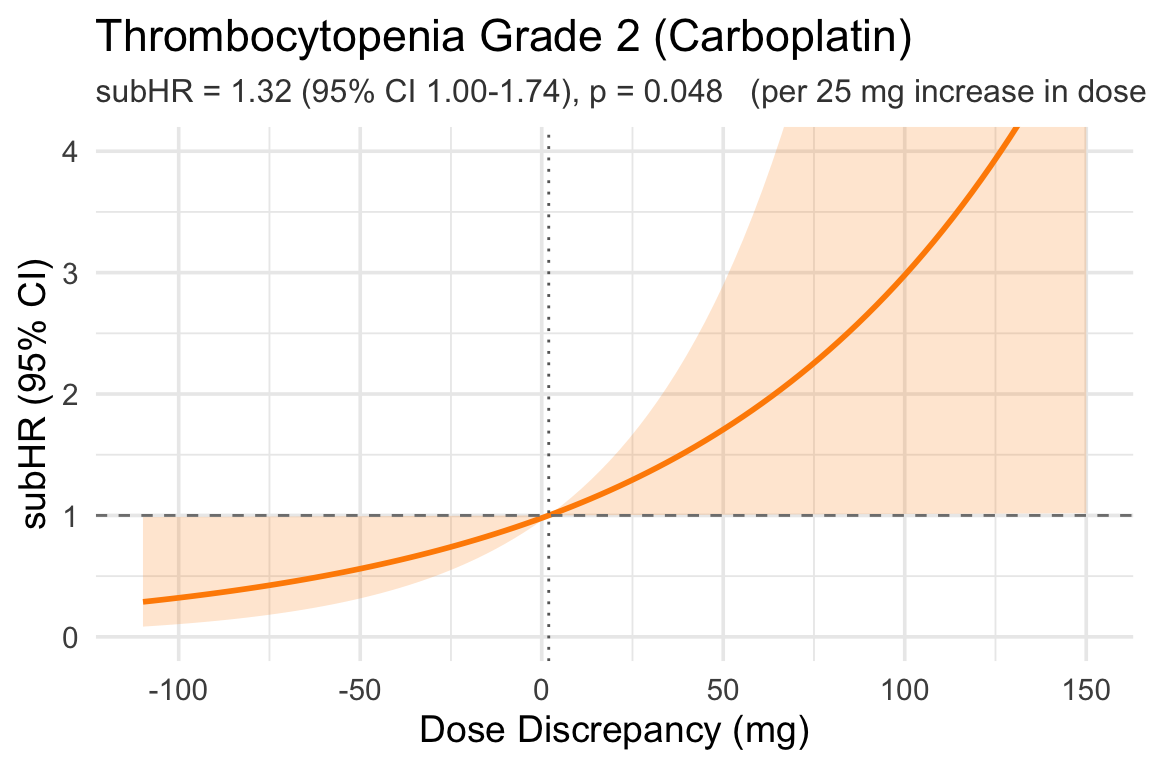
dose_discrep_per25increase 121 1.35 1.11, 1.63 0.002 121 1.32 1.00, 1.74 0.048
age 121 0.98 0.93, 1.03 0.350 121 1.00 0.93, 1.07 0.970
sex 121


121


    Female
— —

— —
    Male
1.04 0.40, 2.74 0.930
0.99 0.39, 2.46 0.980
ecog_score 121 1.93 1.23, 3.03 0.004 121 1.27 0.58, 2.78 0.550
ici 121 1.10 0.42, 2.89 0.850 121 1.39 0.41, 4.75 0.600
cockcroft 121 1.01 1.00, 1.03 0.095 121 1.00 0.98, 1.02 0.980
pre_PLT_45days 121 1.00 0.99, 1.00 0.670 121 1.00 0.99, 1.00 0.460
1 HR = Hazard Ratio, CI = Confidence Interval

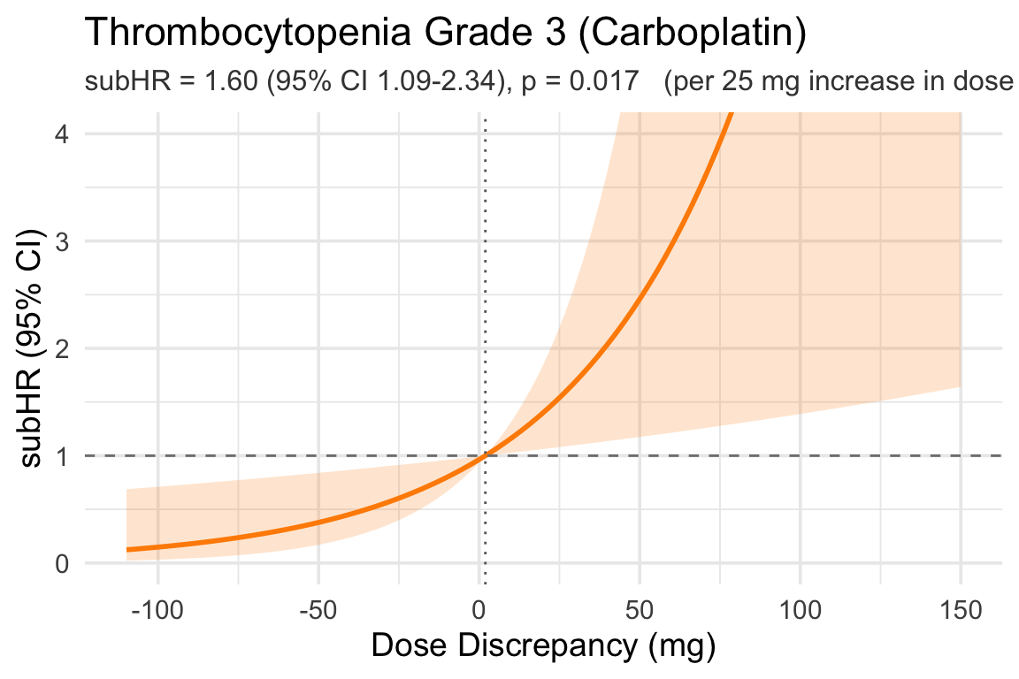
7.4 Thrombocytopenia Grade 3

Code
fg_model("cmp_time_throm_3", "cmp_status_throm_3", "dose_discrep_per25increase", "pre_PLT_45days", "cockcroft")
Characteristic
Univariable
Multivariable
N HR1 95% CI1 p-value N HR1 95% CI1 p-value
dose_discrep_per25increase 121 1.54 1.18, 2.01 0.002 121 1.60 1.09, 2.34 0.017
age 121 1.00 0.94, 1.06 0.980 121 1.05 0.96, 1.15 0.310
sex 121


121


    Female
— —

— —
    Male
2.53 0.67, 9.54 0.170
1.55 0.35, 6.92 0.570
ecog_score 121 1.75 1.06, 2.88 0.029 121 0.79 0.26, 2.40 0.670
ici 121 1.69 0.48, 5.89 0.410 121 1.32 0.27, 6.39 0.730
cockcroft 121 1.02 1.00, 1.04 0.027 121 1.01 0.98, 1.04 0.530
pre_PLT_45days 121 1.00 0.99, 1.01 0.900 121 1.00 0.99, 1.01 0.700
1 HR = Hazard Ratio, CI = Confidence Interval

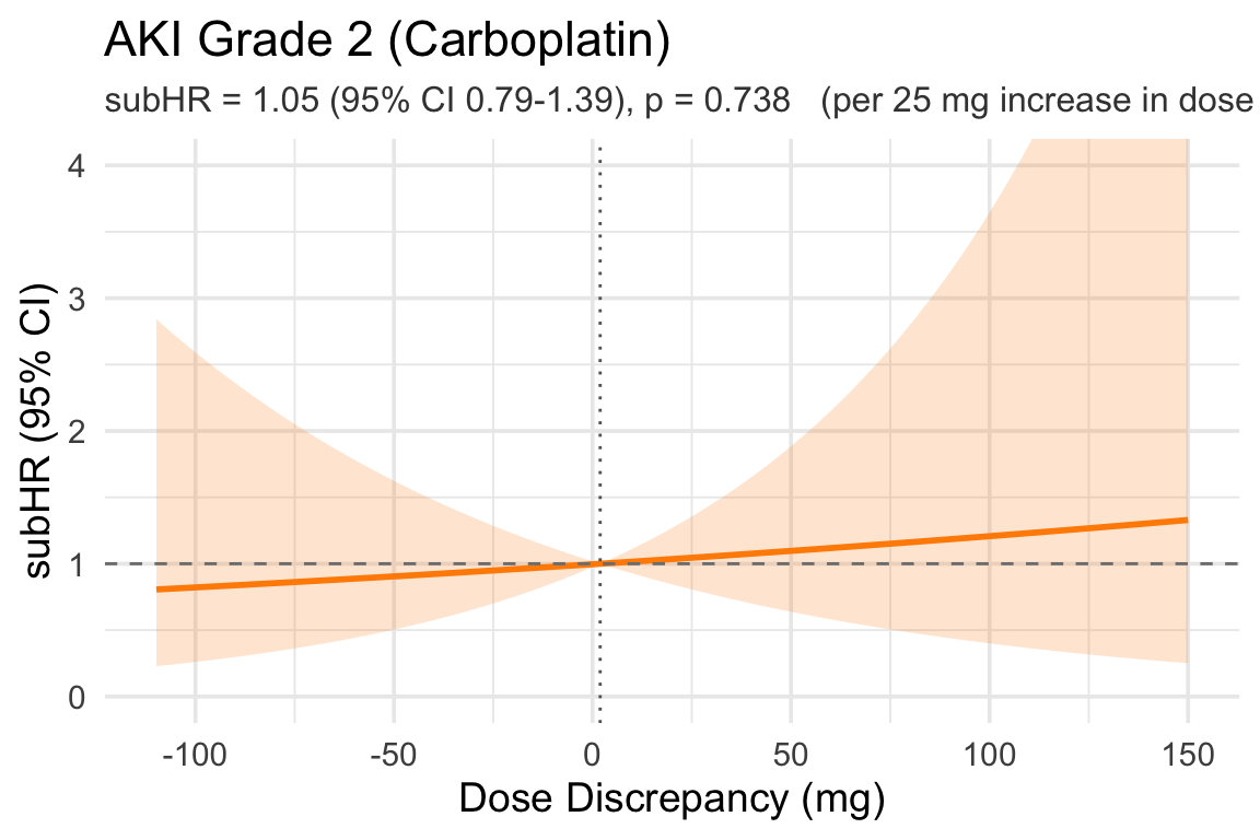
7.5 AKI Grade 2

Code
fg_model("cmp_time_aki_2", "cmp_status_aki_2", "dose_discrep_per25increase", egfr_adj = "cockcroft")
Characteristic
Univariable
Multivariable
N HR1 95% CI1 p-value N HR1 95% CI1 p-value
dose_discrep_per25increase 121 1.20 0.96, 1.50 0.110 121 1.05 0.79, 1.39 0.740
age 121 1.00 0.95, 1.06 0.890 121 1.01 0.90, 1.13 0.850
sex 121


121


    Female
— —

— —
    Male
1.74 0.42, 7.18 0.440
1.62 0.29, 8.88 0.580
ecog_score 121 2.33 1.29, 4.22 0.005 121 2.48 0.83, 7.42 0.100
ici 121 1.88 0.46, 7.71 0.380 121 2.34 0.46, 11.9 0.300
cockcroft 121 1.01 1.00, 1.03 0.062 121 1.01 0.99, 1.02 0.520
1 HR = Hazard Ratio, CI = Confidence Interval

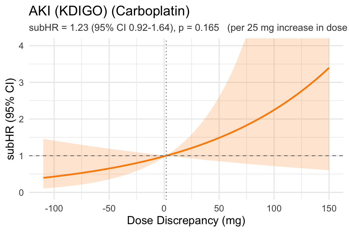
7.6 AKI (KDIGO)

Code
fg_model("cmp_time_aki_kdigo", "cmp_status_aki_kdigo", "dose_discrep_per25increase", egfr_adj = "cockcroft")
Characteristic
Univariable
Multivariable
N HR1 95% CI1 p-value N HR1 95% CI1 p-value
dose_discrep_per25increase 121 1.22 1.02, 1.47 0.031 121 1.23 0.92, 1.64 0.160
age 121 1.02 0.97, 1.06 0.540 121 1.04 0.94, 1.14 0.450
sex 121


121


    Female
— —

— —
    Male
1.24 0.38, 4.00 0.720
0.98 0.21, 4.62 0.980
ecog_score 121 1.69 0.90, 3.18 0.100 121 1.33 0.46, 3.87 0.600
ici 121 1.98 0.59, 6.68 0.270 121 2.03 0.57, 7.20 0.270
cockcroft 121 1.01 0.99, 1.02 0.220 121 1.00 0.99, 1.02 0.720
1 HR = Hazard Ratio, CI = Confidence Interval

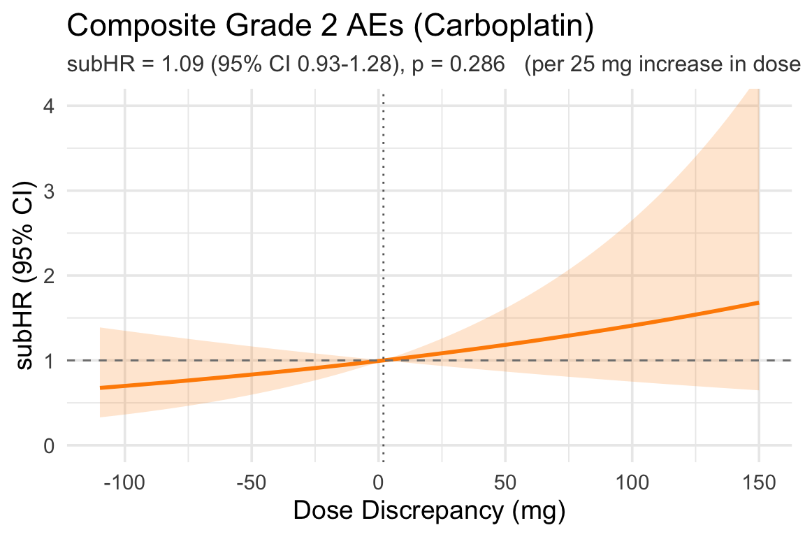
7.7 Composite Grade 2 AEs

Code
fg_model("cmp_time_grade_2_aes", "cmp_status_grade_2_aes", "dose_discrep_per25increase", pre_labs = c("pre_HGB_45days", "pre_PLT_45days"), egfr_adj = "cockcroft")
Characteristic
Univariable
Multivariable
N HR1 95% CI1 p-value N HR1 95% CI1 p-value
dose_discrep_per25increase 121 1.19 1.06, 1.34 0.004 121 1.09 0.93, 1.28 0.290
age 121 0.99 0.96, 1.02 0.600 121 1.00 0.96, 1.04 0.960
sex 121


121


    Female
— —

— —
    Male
1.11 0.63, 1.95 0.710
1.67 0.91, 3.06 0.095
ecog_score 121 1.51 1.03, 2.21 0.035 121 1.37 0.83, 2.26 0.220
ici 121 0.83 0.47, 1.48 0.530 121 1.14 0.62, 2.09 0.680
cockcroft 121 1.00 0.99, 1.01 0.570 121 1.00 0.99, 1.01 0.700
pre_HGB_45days 121 0.58 0.49, 0.69 <0.001 121 0.56 0.45, 0.71 <0.001
pre_PLT_45days 121 1.00 1.00, 1.00 0.470 121 1.00 1.00, 1.00 0.350
1 HR = Hazard Ratio, CI = Confidence Interval

7.8 Composite Grade 3 AEs

Code
fg_model("cmp_time_grade_3_aes", "cmp_status_grade_3_aes", "dose_discrep_per25increase", pre_labs = c("pre_HGB_45days", "pre_PLT_45days"), egfr_adj = "cockcroft")
Characteristic
Univariable
Multivariable
N HR1 95% CI1 p-value N HR1 95% CI1 p-value
dose_discrep_per25increase 121 1.32 1.10, 1.60 0.003 121 1.07 0.83, 1.38 0.590
age 121 1.00 0.95, 1.05 0.940 121 1.01 0.94, 1.09 0.730
sex 121


121


    Female
— —

— —
    Male
1.83 0.68, 4.93 0.230
1.85 0.54, 6.31 0.330
ecog_score 121 1.72 1.04, 2.82 0.033 121 1.68 0.66, 4.29 0.280
ici 121 1.15 0.44, 3.02 0.780 121 1.11 0.37, 3.28 0.860
cockcroft 121 1.01 1.00, 1.03 0.110 121 1.00 0.98, 1.03 0.700
pre_HGB_45days 121 0.48 0.35, 0.64 <0.001 121 0.51 0.35, 0.74 <0.001
pre_PLT_45days 121 1.01 1.00, 1.01 0.001 121 1.00 1.00, 1.01 0.820
1 HR = Hazard Ratio, CI = Confidence Interval

7.9 Overall Hospitalization

Code
fg_model("cmp_time_any_hosp", "cmp_status_any_hosp", "dose_discrep_per25increase", egfr_adj = "cockcroft")
Characteristic
Univariable
Multivariable
N HR1 95% CI1 p-value N HR1 95% CI1 p-value
dose_discrep_per25increase 121 1.23 1.07, 1.41 0.004 121 1.33 1.13, 1.57 <0.001
age 121 1.02 0.97, 1.07 0.540 121 1.04 0.98, 1.10 0.180
sex 121


121


    Female
— —

— —
    Male
1.15 0.56, 2.36 0.700
1.15 0.57, 2.31 0.700
ecog_score 121 1.45 0.89, 2.36 0.130 121 1.08 0.60, 1.94 0.800
ici 121 0.91 0.44, 1.88 0.800 121 0.88 0.38, 2.03 0.760
cockcroft 121 1.00 0.99, 1.01 0.680 121 1.0 0.98, 1.01 0.520
1 HR = Hazard Ratio, CI = Confidence Interval

7.11 90-Day Death (Cox PH)

Code
cox_model("time_to_death_90", "death_90", "dose_discrep_per25increase", egfr_adj = "cockcroft")
Characteristic
Univariable
Multivariable
N HR1 95% CI1 p-value N HR1 95% CI1 p-value
dose_discrep_per25increase 121 1.41 1.11, 1.81 0.006 121 1.40 1.04, 1.87 0.026
age 121 1.02 0.95, 1.10 0.539 121 1.06 0.96, 1.16 0.270
sex 121


121


    Female
— —

— —
    Male
1.60 0.45, 5.66 0.468
2.05 0.50, 8.39 0.319
ecog_score 121 3.85 1.91, 7.76 <0.001 121 3.65 1.47, 9.11 0.005
ici 121 0.73 0.21, 2.60 0.632 121 1.16 0.27, 5.08 0.842
cockcroft 121 1.01 0.99, 1.03 0.357 121 0.99 0.97, 1.01 0.562
1 HR = Hazard Ratio, CI = Confidence Interval

8 Cause-Specific Hazard Models — Dose Discrepancy per 25 mg (Carboplatin)

8.1 Anemia Grade 2

Code
csh_model("cmp_time_anemia_2", "cmp_status_anemia_2", "dose_discrep_per25increase", "pre_HGB_45days")
Characteristic N HR1 95% CI1 p-value
dose_discrep_per25increase 121 1.18 1.00, 1.40 0.055
age 121 1.02 0.98, 1.06 0.297
sex 121


    Female
— —
    Male
1.44 0.75, 2.74 0.273
ecog_score 121 1.61 0.99, 2.64 0.056
ici 121 0.98 0.51, 1.85 0.939
cockcroft 121 0.99 0.98, 1.00 0.156
pre_HGB_45days 121 0.46 0.36, 0.61 <0.001
1 HR = Hazard Ratio, CI = Confidence Interval

8.2 Anemia Grade 3

Code
csh_model("cmp_time_anemia_3", "cmp_status_anemia_3", "dose_discrep_per25increase", "pre_HGB_45days")
Characteristic N HR1 95% CI1 p-value
dose_discrep_per25increase 121 1.05 0.81, 1.36 0.699
age 121 1.04 0.96, 1.12 0.342
sex 121


    Female
— —
    Male
2.01 0.57, 7.07 0.274
ecog_score 121 2.85 1.13, 7.18 0.026
ici 121 1.30 0.40, 4.25 0.660
cockcroft 121 1.00 0.97, 1.02 0.671
pre_HGB_45days 121 0.38 0.23, 0.62 <0.001
1 HR = Hazard Ratio, CI = Confidence Interval

8.3 Thrombocytopenia Grade 2

Code
csh_model("cmp_time_throm_2", "cmp_status_throm_2", "dose_discrep_per25increase", "pre_PLT_45days")
Characteristic N HR1 95% CI1 p-value
dose_discrep_per25increase 121 1.38 1.06, 1.80 0.019
age 121 1.01 0.94, 1.08 0.836
sex 121


    Female
— —
    Male
1.02 0.35, 3.01 0.969
ecog_score 121 1.35 0.60, 3.04 0.475
ici 121 1.38 0.44, 4.31 0.576
cockcroft 121 1.00 0.98, 1.02 0.989
pre_PLT_45days 121 1.00 0.99, 1.00 0.396
1 HR = Hazard Ratio, CI = Confidence Interval

8.4 Thrombocytopenia Grade 3

Code
csh_model("cmp_time_throm_3", "cmp_status_throm_3", "dose_discrep_per25increase", "pre_PLT_45days")
Characteristic N HR1 95% CI1 p-value
dose_discrep_per25increase 121 1.69 1.19, 2.40 0.003
age 121 1.05 0.96, 1.16 0.291
sex 121


    Female
— —
    Male
1.73 0.37, 8.12 0.486
ecog_score 121 0.91 0.32, 2.56 0.851
ici 121 1.28 0.31, 5.30 0.729
cockcroft 121 1.01 0.99, 1.03 0.452
pre_PLT_45days 121 1.00 0.99, 1.00 0.599
1 HR = Hazard Ratio, CI = Confidence Interval

8.5 AKI Grade 2

Code
csh_model("cmp_time_aki_2", "cmp_status_aki_2", "dose_discrep_per25increase")
Characteristic N HR1 95% CI1 p-value
dose_discrep_per25increase 121 1.08 0.77, 1.52 0.645
age 121 1.01 0.92, 1.12 0.806
sex 121


    Female
— —
    Male
1.70 0.37, 7.77 0.493
ecog_score 121 2.62 0.82, 8.42 0.105
ici 121 2.35 0.46, 12.1 0.305
cockcroft 121 1.01 0.98, 1.03 0.636
1 HR = Hazard Ratio, CI = Confidence Interval

8.6 AKI (KDIGO)

Code
csh_model("cmp_time_aki_kdigo", "cmp_status_aki_kdigo", "dose_discrep_per25increase")
Characteristic N HR1 95% CI1 p-value
dose_discrep_per25increase 121 1.26 0.93, 1.70 0.135
age 121 1.04 0.96, 1.13 0.361
sex 121


    Female
— —
    Male
1.00 0.28, 3.65 0.997
ecog_score 121 1.42 0.50, 3.99 0.507
ici 121 1.95 0.51, 7.43 0.326
cockcroft 121 1.00 0.98, 1.02 0.782
1 HR = Hazard Ratio, CI = Confidence Interval

8.7 Composite Grade 2 AEs

Code
csh_model("cmp_time_grade_2_aes", "cmp_status_grade_2_aes", "dose_discrep_per25increase", c("pre_HGB_45days", "pre_PLT_45days"))
Characteristic N HR1 95% CI1 p-value
dose_discrep_per25increase 121 1.13 0.96, 1.32 0.138
age 121 1.01 0.97, 1.05 0.642
sex 121


    Female
— —
    Male
1.56 0.84, 2.92 0.161
ecog_score 121 1.58 1.00, 2.48 0.048
ici 121 1.07 0.57, 2.04 0.826
cockcroft 121 1.00 0.98, 1.01 0.403
pre_HGB_45days 121 0.50 0.38, 0.65 <0.001
pre_PLT_45days 121 1.00 0.99, 1.00 0.129
1 HR = Hazard Ratio, CI = Confidence Interval

8.8 Composite Grade 3 AEs

Code
csh_model("cmp_time_grade_3_aes", "cmp_status_grade_3_aes", "dose_discrep_per25increase", c("pre_HGB_45days", "pre_PLT_45days"))
Characteristic N HR1 95% CI1 p-value
dose_discrep_per25increase 121 1.12 0.87, 1.43 0.390
age 121 1.02 0.95, 1.09 0.542
sex 121


    Female
— —
    Male
1.99 0.58, 6.74 0.271
ecog_score 121 2.13 0.92, 4.90 0.076
ici 121 0.91 0.30, 2.71 0.860
cockcroft 121 1.00 0.98, 1.02 0.788
pre_HGB_45days 121 0.47 0.30, 0.75 0.001
pre_PLT_45days 121 1.00 1.00, 1.01 0.535
1 HR = Hazard Ratio, CI = Confidence Interval

8.9 Overall Hospitalization

Code
csh_model("cmp_time_any_hosp", "cmp_status_any_hosp", "dose_discrep_per25increase")
Characteristic N HR1 95% CI1 p-value
dose_discrep_per25increase 121 1.37 1.13, 1.65 0.001
age 121 1.05 0.99, 1.10 0.100
sex 121


    Female
— —
    Male
1.12 0.52, 2.42 0.776
ecog_score 121 1.14 0.64, 2.04 0.658
ici 121 0.86 0.39, 1.91 0.716
cockcroft 121 0.99 0.98, 1.01 0.440
1 HR = Hazard Ratio, CI = Confidence Interval

8.11 90-Day Death (Cox PH)

Code
cox_model("time_to_death_90", "death_90", "dose_discrep_per25increase", egfr_adj = "cockcroft")
Characteristic
Univariable
Multivariable
N HR1 95% CI1 p-value N HR1 95% CI1 p-value
dose_discrep_per25increase 121 1.41 1.11, 1.81 0.006 121 1.40 1.04, 1.87 0.026
age 121 1.02 0.95, 1.10 0.539 121 1.06 0.96, 1.16 0.270
sex 121


121


    Female
— —

— —
    Male
1.60 0.45, 5.66 0.468
2.05 0.50, 8.39 0.319
ecog_score 121 3.85 1.91, 7.76 <0.001 121 3.65 1.47, 9.11 0.005
ici 121 0.73 0.21, 2.60 0.632 121 1.16 0.27, 5.08 0.842
cockcroft 121 1.01 0.99, 1.03 0.357 121 0.99 0.97, 1.01 0.562
1 HR = Hazard Ratio, CI = Confidence Interval
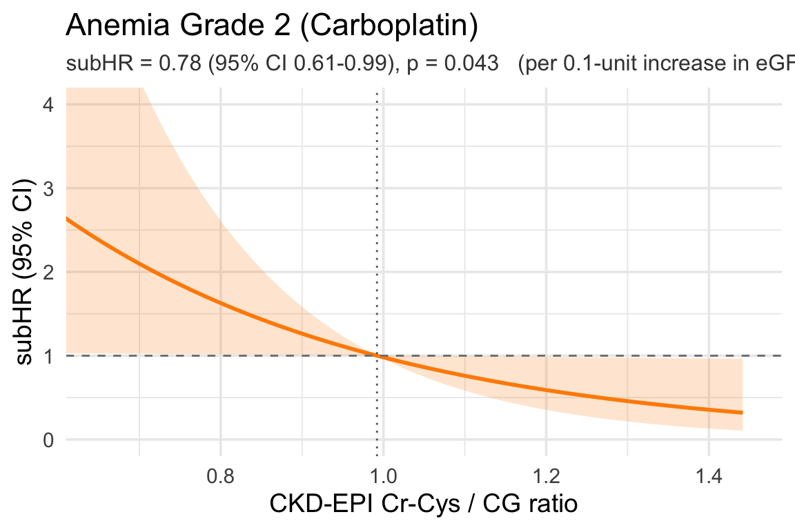
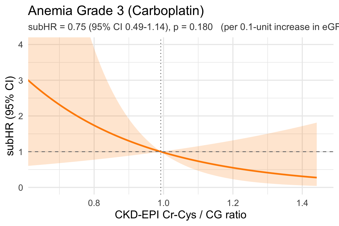
NoteWhy anchor at the median (subHR = 1 at the reference)

Three reasons to anchor at the median:

  1. Interpretability: “A patient with eGFR ratio of 0.8 has ~1.5× the subHR compared to a typical patient (at the median).”
  2. Stability: The median sits in the densest part of the data, so estimates near it have the tightest confidence intervals. The CIs fan out as you move away — you can see this in the plots.
  3. No arbitrary choice: If we picked 1.0 arbitrarily, the plot would look almost identical here (because median ≈ 1), but in cohorts where the median is 0.9 or 1.1, picking 1.0 would either shift or distort the curve without changing the actual model.

9 Linear subHR Curves — eGFR Ratio (raw scale) (Carboplatin)

Code
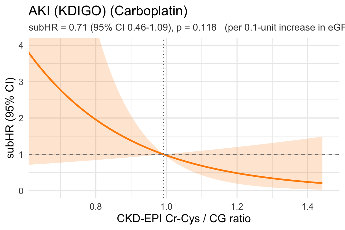
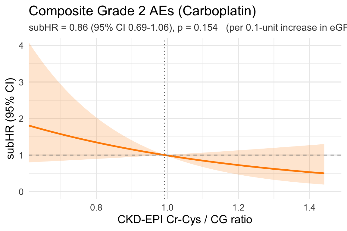
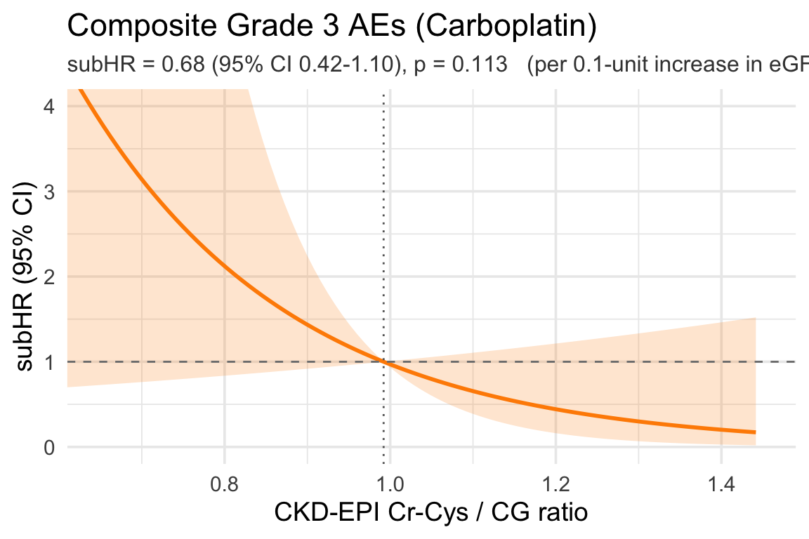
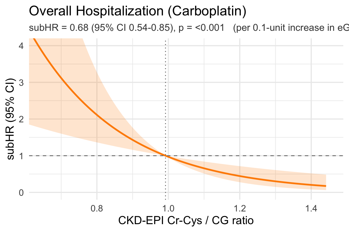
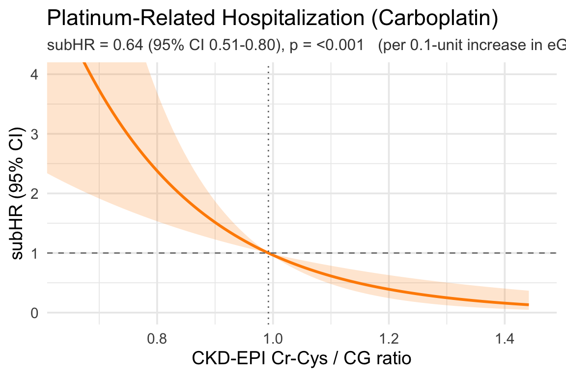
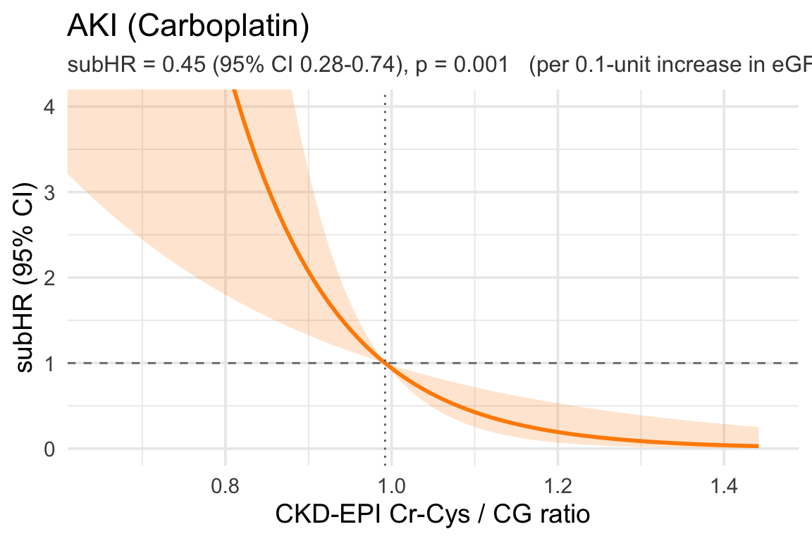
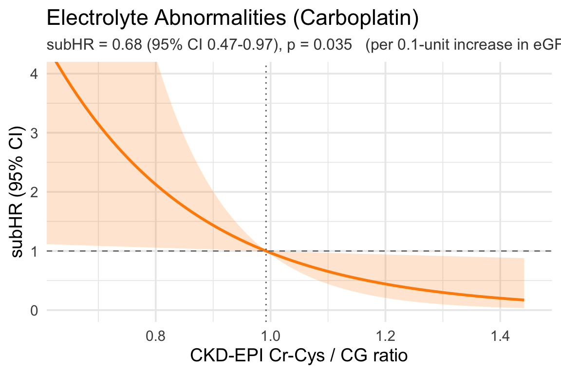
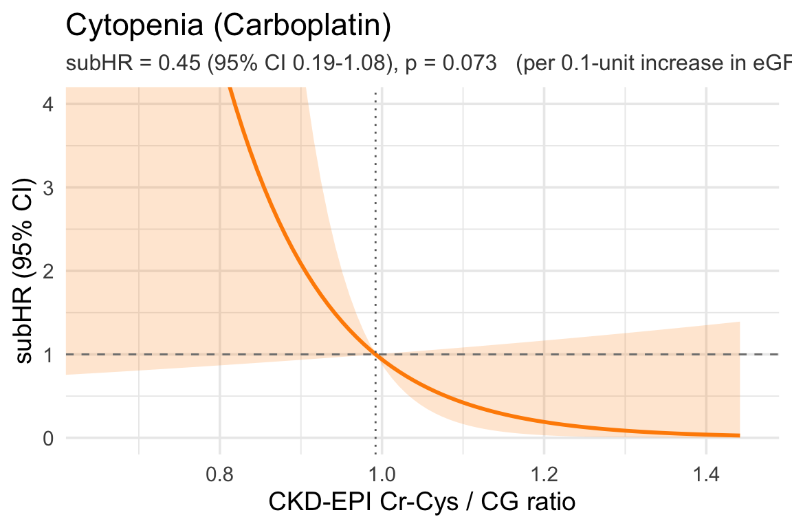
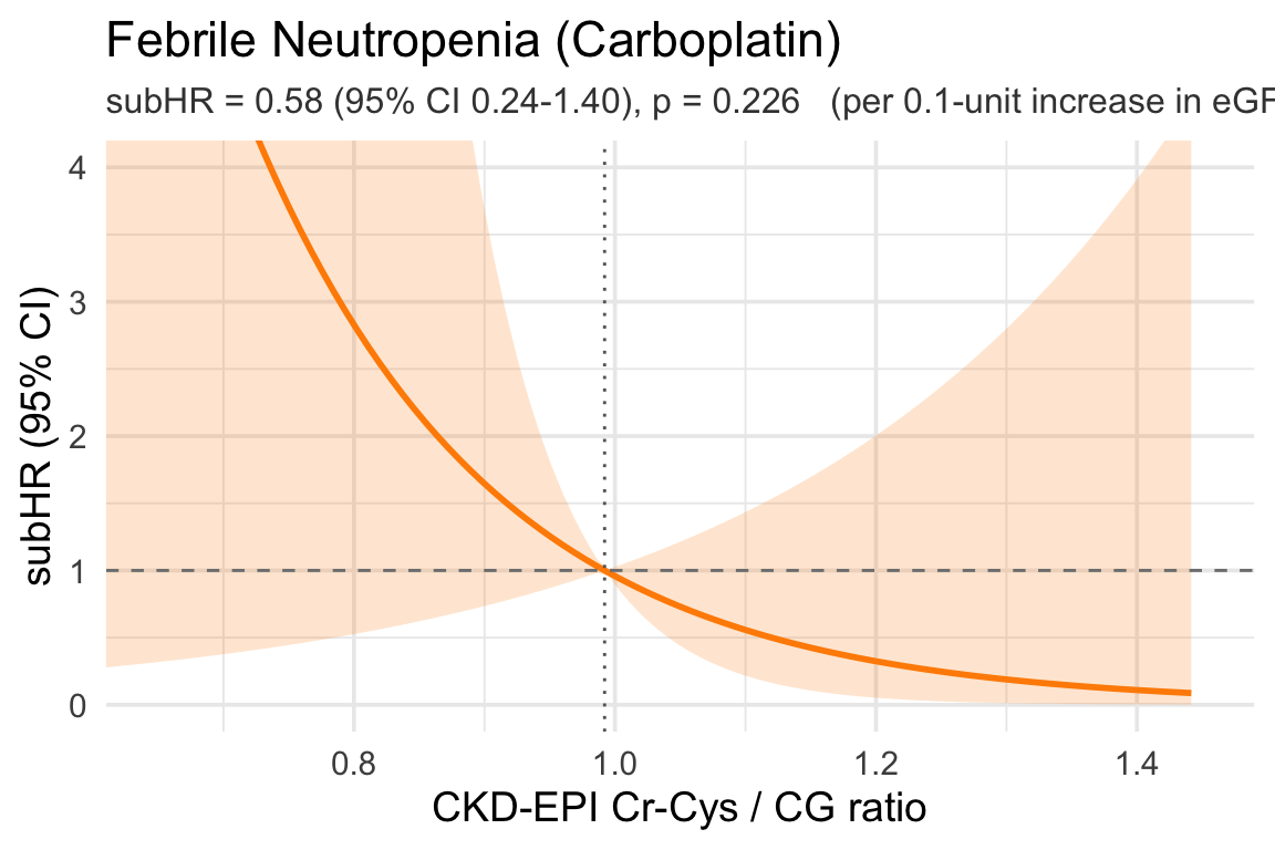
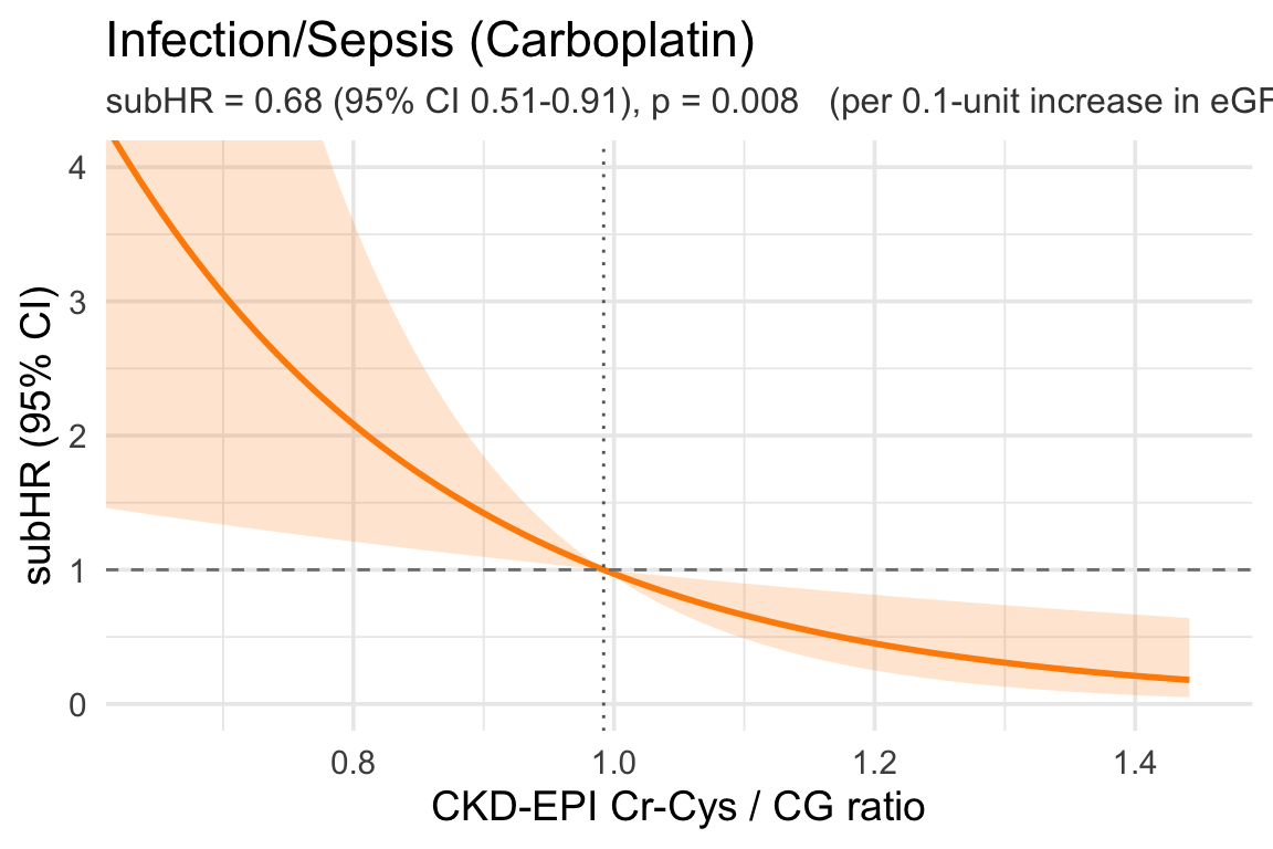
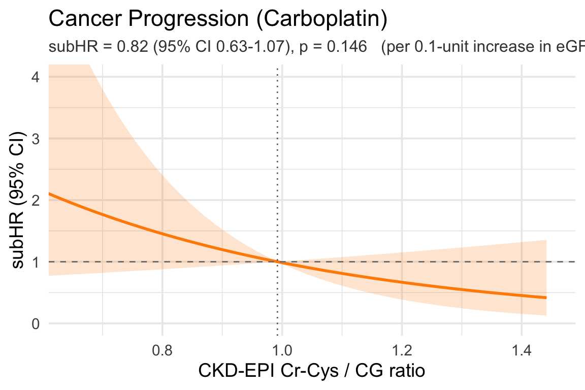
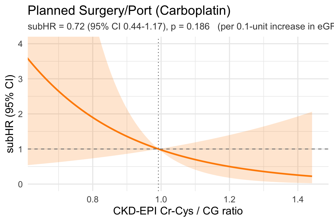
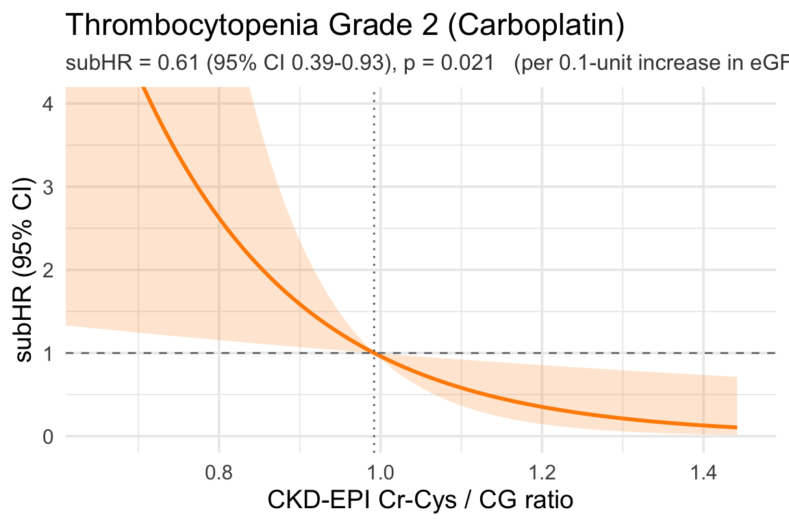
plot_subhr_linear_ratio <- function(time_var, status_var, extra_adj = NULL,
                                    outcome_label) {
  base_adj <- c("age", "sex", "ecog_score", "ici", "cockcroft")
  keep <- c("egfr_ratio", time_var, status_var, base_adj, extra_adj)
  d <- dat %>% dplyr::select(all_of(keep)) %>% tidyr::drop_na()

  adj_df <- d[, c(base_adj, extra_adj), drop = FALSE]
  X_adj <- model.matrix(~ ., data = adj_df)[, -1, drop = FALSE]
  X <- cbind(egfr_ratio = d$egfr_ratio, X_adj)

  stat_num <- suppressWarnings(as.integer(as.character(d[[status_var]])))
  time_num <- as.numeric(d[[time_var]])

  fit <- tryCatch(
    cmprsk::crr(ftime = time_num, fstatus = stat_num,
                cov1 = X, failcode = 1),
    error = function(e) NULL
  )
  if (is.null(fit)) return(.plot_failed(outcome_label))

  beta   <- fit$coef[1]
  V_beta <- fit$var[1, 1]
  subtitle_str <- .hr_subtitle(beta, V_beta, scale = 0.1,
                               hr_type = "subHR",
                               unit_label = "per 0.1-unit increase in eGFR ratio")

  ref_x  <- median(d$egfr_ratio, na.rm = TRUE)
  grid_x <- seq(quantile(d$egfr_ratio, 0.025, na.rm = TRUE),
                quantile(d$egfr_ratio, 0.975, na.rm = TRUE),
                length.out = 100)

  log_hr <- beta * (grid_x - ref_x)
  se     <- sqrt((grid_x - ref_x)^2 * V_beta)

  df_plot <- tibble(
    x     = grid_x,
    subhr = exp(log_hr),
    lcl   = exp(log_hr - 1.96 * se),
    ucl   = exp(log_hr + 1.96 * se)
  )

  ggplot(df_plot, aes(x = x, y = subhr)) +
    geom_ribbon(aes(ymin = lcl, ymax = ucl), alpha = 0.2, fill = "darkorange") +
    geom_line(color = "darkorange", linewidth = 1) +
    geom_hline(yintercept = 1, linetype = "dashed", color = "grey50") +
    geom_vline(xintercept = ref_x, linetype = "dotted", color = "grey40") +
    labs(x = "CKD-EPI Cr-Cys / CG ratio",
         y = "subHR (95% CI)",
         title = outcome_label,
         subtitle = subtitle_str) +
    coord_cartesian(xlim = c(0.65, 1.45), ylim = c(0, 4)) +
    theme_minimal(base_size = 14) +
    theme(plot.subtitle = element_text(size = 12, color = "grey25")) -> p
  .save_plot_pptx(p)
  p
}
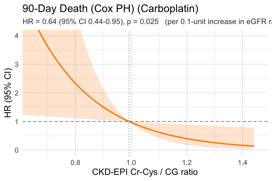
plot_cox_linear_ratio <- function(time_var, status_var, extra_adj = NULL,
                                  outcome_label) {
  base_adj <- c("age", "sex", "ecog_score", "ici", "cockcroft")
  keep <- c("egfr_ratio", time_var, status_var, base_adj, extra_adj)
  d <- dat %>% dplyr::select(all_of(keep)) %>% tidyr::drop_na()

  fmla <- as.formula(paste0(
    "Surv(", time_var, ", ", status_var, ") ~ egfr_ratio + ",
    paste(c(base_adj, extra_adj), collapse = " + ")
  ))
  fit <- tryCatch(survival::coxph(fmla, data = d), error = function(e) NULL)
  if (is.null(fit)) return(.plot_failed(outcome_label))

  beta   <- coef(fit)["egfr_ratio"]
  V_beta <- vcov(fit)["egfr_ratio", "egfr_ratio"]
  subtitle_str <- .hr_subtitle(beta, V_beta, scale = 0.1,
                               hr_type = "HR",
                               unit_label = "per 0.1-unit increase in eGFR ratio (Cox PH)")

  ref_x  <- median(d$egfr_ratio, na.rm = TRUE)
  grid_x <- seq(quantile(d$egfr_ratio, 0.025, na.rm = TRUE),
                quantile(d$egfr_ratio, 0.975, na.rm = TRUE),
                length.out = 100)

  log_hr <- beta * (grid_x - ref_x)
  se     <- sqrt((grid_x - ref_x)^2 * V_beta)

  df_plot <- tibble(
    x   = grid_x,
    hr  = exp(log_hr),
    lcl = exp(log_hr - 1.96 * se),
    ucl = exp(log_hr + 1.96 * se)
  )

  ggplot(df_plot, aes(x = x, y = hr)) +
    geom_ribbon(aes(ymin = lcl, ymax = ucl), alpha = 0.2, fill = "darkorange") +
    geom_line(color = "darkorange", linewidth = 1) +
    geom_hline(yintercept = 1, linetype = "dashed", color = "grey50") +
    geom_vline(xintercept = ref_x, linetype = "dotted", color = "grey40") +
    labs(x = "CKD-EPI Cr-Cys / CG ratio",
         y = "HR (95% CI)",
         title = outcome_label,
         subtitle = subtitle_str) +
    coord_cartesian(xlim = c(0.65, 1.45), ylim = c(0, 4)) +
    theme_minimal(base_size = 14) +
    theme(plot.subtitle = element_text(size = 12, color = "grey25")) -> p
  .save_plot_pptx(p)
  p
}
9.1 Anemia Grade 2

Code
plot_subhr_linear_ratio("cmp_time_anemia_2", "cmp_status_anemia_2",
                        "pre_HGB_45days", "Anemia Grade 2 (Carboplatin)")

9.2 Anemia Grade 3

Code
plot_subhr_linear_ratio("cmp_time_anemia_3", "cmp_status_anemia_3",
                        "pre_HGB_45days", "Anemia Grade 3 (Carboplatin)")

9.3 Thrombocytopenia Grade 2

Code
plot_subhr_linear_ratio("cmp_time_throm_2", "cmp_status_throm_2",
                        "pre_PLT_45days", "Thrombocytopenia Grade 2 (Carboplatin)")

9.4 Thrombocytopenia Grade 3

Code
plot_subhr_linear_ratio("cmp_time_throm_3", "cmp_status_throm_3",
                        "pre_PLT_45days", "Thrombocytopenia Grade 3 (Carboplatin)")

9.5 AKI Grade 2

Code
plot_subhr_linear_ratio("cmp_time_aki_2", "cmp_status_aki_2",
                        NULL, "AKI Grade 2 (Carboplatin)")

9.6 AKI (KDIGO)

Code
plot_subhr_linear_ratio("cmp_time_aki_kdigo", "cmp_status_aki_kdigo",
                        NULL, "AKI (KDIGO) (Carboplatin)")

9.7 Composite Grade 2 AEs

Code
plot_subhr_linear_ratio("cmp_time_grade_2_aes", "cmp_status_grade_2_aes",
                        c("pre_HGB_45days", "pre_PLT_45days"), "Composite Grade 2 AEs (Carboplatin)")

9.8 Composite Grade 3 AEs

Code
plot_subhr_linear_ratio("cmp_time_grade_3_aes", "cmp_status_grade_3_aes",
                        c("pre_HGB_45days", "pre_PLT_45days"), "Composite Grade 3 AEs (Carboplatin)")

9.9 Overall Hospitalization

Code
plot_subhr_linear_ratio("cmp_time_any_hosp", "cmp_status_any_hosp",
                        NULL, "Overall Hospitalization (Carboplatin)")

9.11 90-Day Death (Cox PH)

Code
plot_cox_linear_ratio("time_to_death_90", "death_90",
                      NULL, "90-Day Death (Cox PH) (Carboplatin)")

10 Linear subHR Curves — eGFR Discrepancy (raw scale) (Carboplatin)

Code
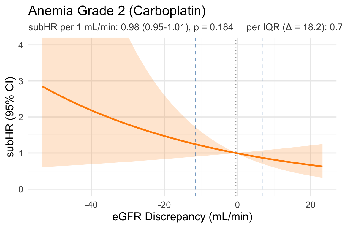
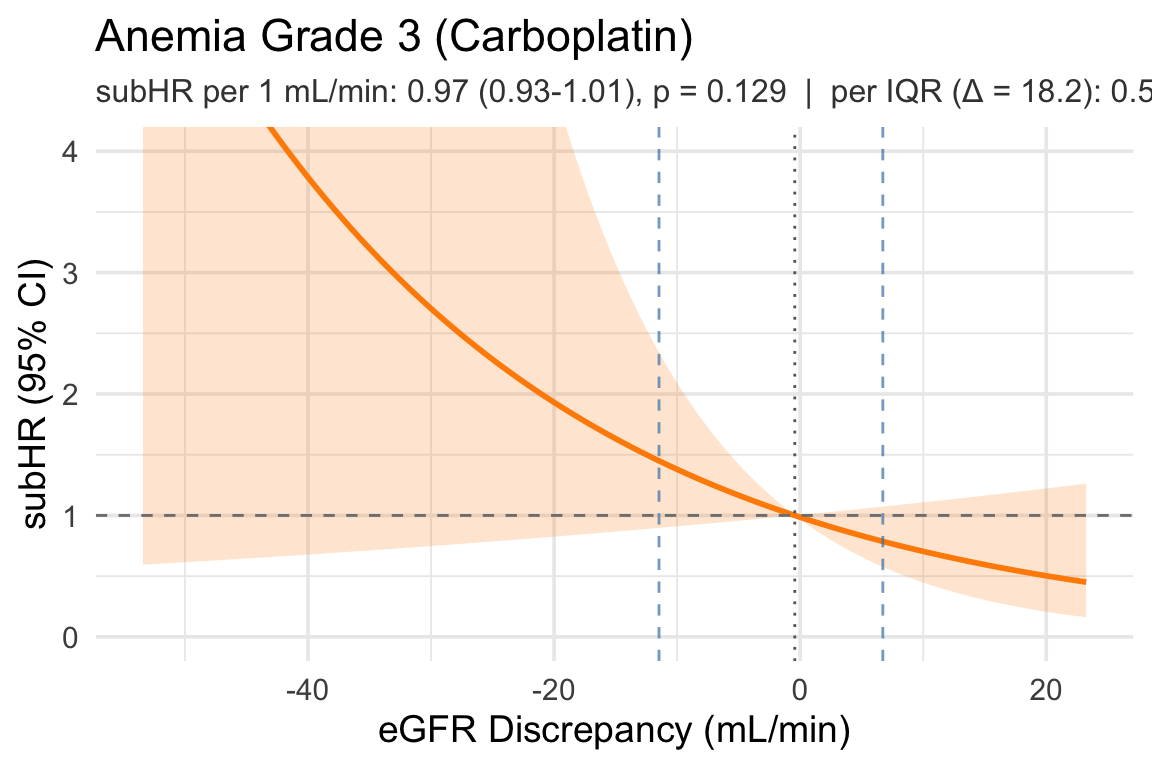
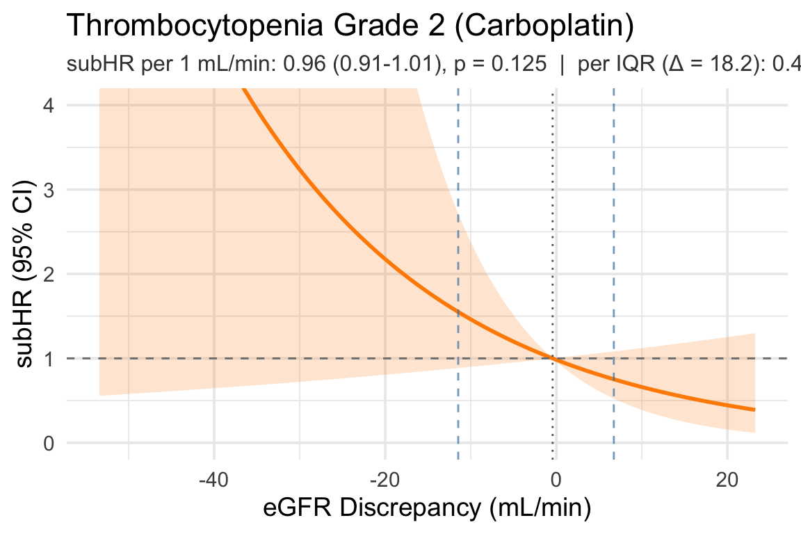
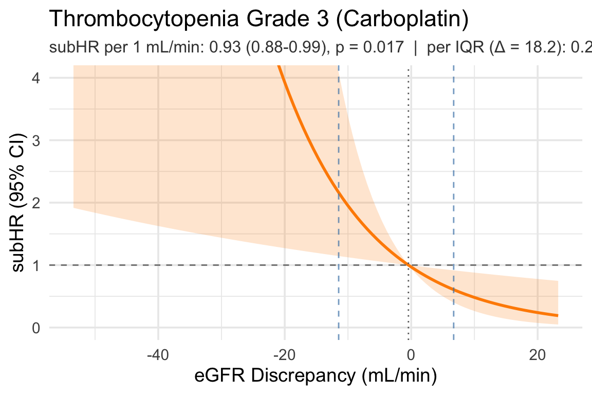
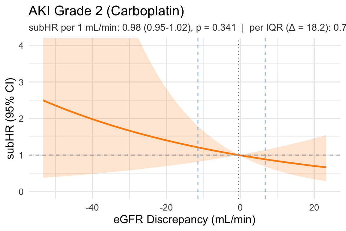
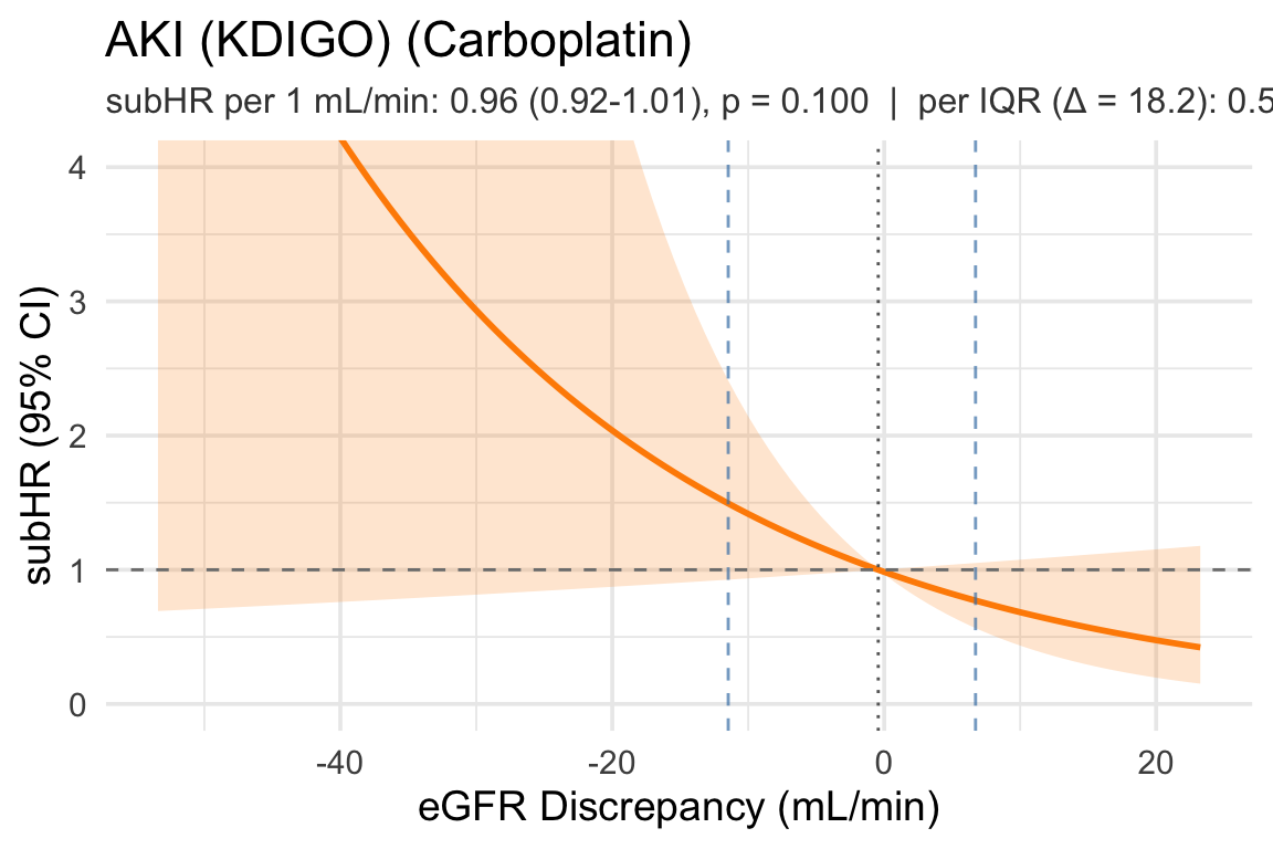
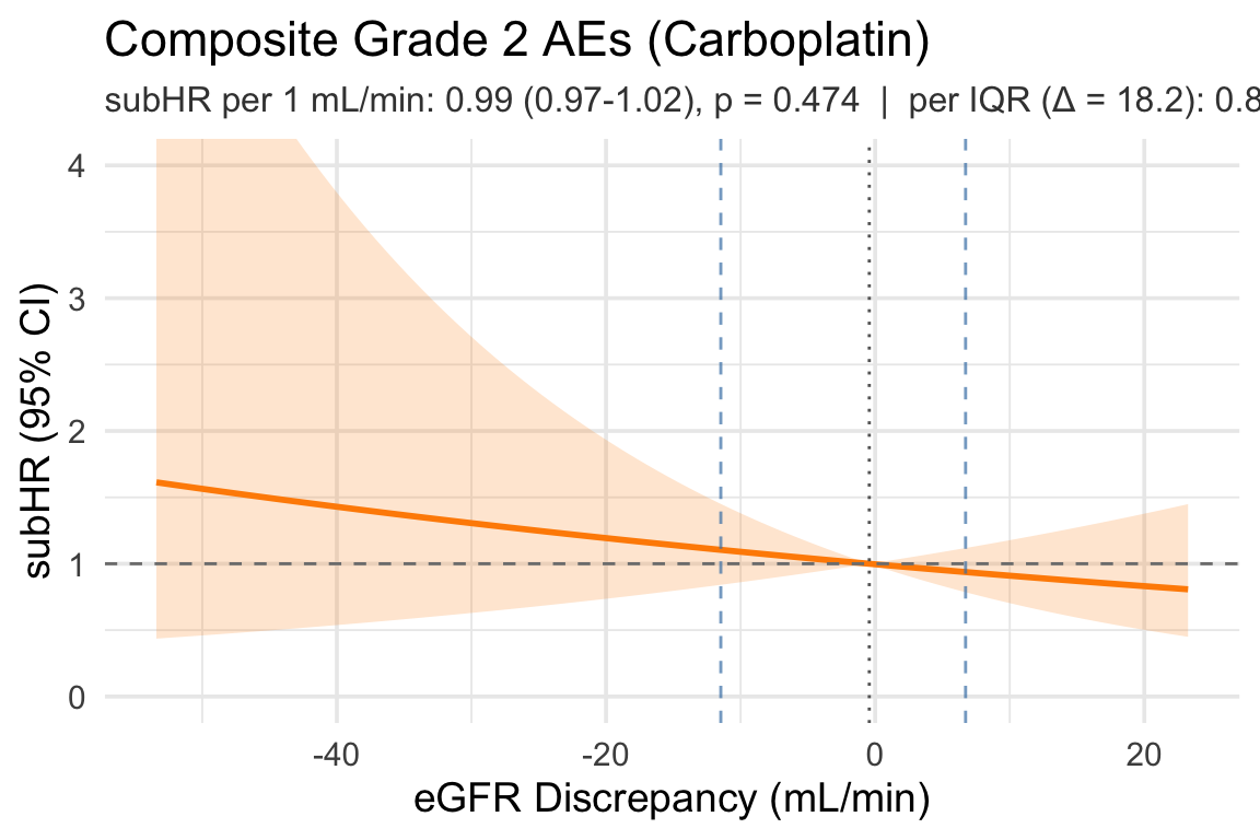
plot_subhr_linear_egfrdisc <- function(time_var, status_var, extra_adj = NULL,
                                       outcome_label) {
  base_adj <- c("age", "sex", "ecog_score", "ici", "cockcroft")
  keep <- c("egfr_discrepancy", time_var, status_var, base_adj, extra_adj)
  d <- dat %>% dplyr::select(all_of(keep)) %>% tidyr::drop_na()

  adj_df <- d[, c(base_adj, extra_adj), drop = FALSE]
  X_adj <- model.matrix(~ ., data = adj_df)[, -1, drop = FALSE]
  X <- cbind(egfr_discrepancy = d$egfr_discrepancy, X_adj)

  stat_num <- suppressWarnings(as.integer(as.character(d[[status_var]])))
  time_num <- as.numeric(d[[time_var]])

  fit <- tryCatch(
    cmprsk::crr(ftime = time_num, fstatus = stat_num,
                cov1 = X, failcode = 1),
    error = function(e) NULL
  )
  if (is.null(fit)) return(.plot_failed(outcome_label))

  beta   <- fit$coef[1]
  V_beta <- fit$var[1, 1]
  se_b   <- sqrt(V_beta)

  q1    <- as.numeric(quantile(d$egfr_discrepancy, 0.25, na.rm = TRUE))
  q3    <- as.numeric(quantile(d$egfr_discrepancy, 0.75, na.rm = TRUE))
  iqr_w <- q3 - q1
  hr1   <- exp(beta);             hr1_l <- exp(beta - 1.96 * se_b);             hr1_u <- exp(beta + 1.96 * se_b)
  hri   <- exp(beta * iqr_w);     hri_l <- exp(beta * iqr_w - 1.96 * abs(iqr_w) * se_b); hri_u <- exp(beta * iqr_w + 1.96 * abs(iqr_w) * se_b)
  pval  <- 2 * (1 - pnorm(abs(beta / se_b)))
  p_str <- ifelse(pval < 0.001, "<0.001", sprintf("%.3f", pval))
  subtitle_str <- sprintf(
    "subHR per 1 mL/min: %.2f (%.2f-%.2f), p = %s  |  per IQR (Δ = %.1f): %.2f (%.2f-%.2f)  |  IQR: [%.1f, %.1f]",
    hr1, hr1_l, hr1_u, p_str, iqr_w, hri, hri_l, hri_u, q1, q3)

  ref_x  <- median(d$egfr_discrepancy, na.rm = TRUE)
  grid_x <- seq(quantile(d$egfr_discrepancy, 0.025, na.rm = TRUE),
                quantile(d$egfr_discrepancy, 0.975, na.rm = TRUE),
                length.out = 100)

  log_hr <- beta * (grid_x - ref_x)
  se     <- sqrt((grid_x - ref_x)^2 * V_beta)

  df_plot <- tibble(
    x     = grid_x,
    subhr = exp(log_hr),
    lcl   = exp(log_hr - 1.96 * se),
    ucl   = exp(log_hr + 1.96 * se)
  )

  ggplot(df_plot, aes(x = x, y = subhr)) +
    geom_ribbon(aes(ymin = lcl, ymax = ucl), alpha = 0.2, fill = "darkorange") +
    geom_line(color = "darkorange", linewidth = 1) +
    geom_hline(yintercept = 1, linetype = "dashed", color = "grey50") +
    geom_vline(xintercept = ref_x, linetype = "dotted", color = "grey40") +
    geom_vline(xintercept = c(q1, q3), linetype = "dashed",
               color = "steelblue", alpha = 0.7) +
    labs(x = "eGFR Discrepancy (mL/min)",
         y = "subHR (95% CI)",
         title = outcome_label,
         subtitle = subtitle_str) +
    coord_cartesian(ylim = c(0, 4)) +
    theme_minimal(base_size = 14) +
    theme(plot.subtitle = element_text(size = 12, color = "grey25")) -> p
  .save_plot_pptx(p)
  p
}
plot_cox_linear_egfrdisc <- function(time_var, status_var, extra_adj = NULL,
                                     outcome_label) {
  base_adj <- c("age", "sex", "ecog_score", "ici", "cockcroft")
  keep <- c("egfr_discrepancy", time_var, status_var, base_adj, extra_adj)
  d <- dat %>% dplyr::select(all_of(keep)) %>% tidyr::drop_na()

  fmla <- as.formula(paste0(
    "Surv(", time_var, ", ", status_var, ") ~ egfr_discrepancy + ",
    paste(c(base_adj, extra_adj), collapse = " + ")
  ))
  fit <- tryCatch(survival::coxph(fmla, data = d), error = function(e) NULL)
  if (is.null(fit)) return(.plot_failed(outcome_label))

  beta   <- coef(fit)["egfr_discrepancy"]
  V_beta <- vcov(fit)["egfr_discrepancy", "egfr_discrepancy"]
  se_b   <- sqrt(V_beta)

  q1    <- as.numeric(quantile(d$egfr_discrepancy, 0.25, na.rm = TRUE))
  q3    <- as.numeric(quantile(d$egfr_discrepancy, 0.75, na.rm = TRUE))
  iqr_w <- q3 - q1
  hr1   <- exp(beta);             hr1_l <- exp(beta - 1.96 * se_b);             hr1_u <- exp(beta + 1.96 * se_b)
  hri   <- exp(beta * iqr_w);     hri_l <- exp(beta * iqr_w - 1.96 * abs(iqr_w) * se_b); hri_u <- exp(beta * iqr_w + 1.96 * abs(iqr_w) * se_b)
  pval  <- 2 * (1 - pnorm(abs(beta / se_b)))
  p_str <- ifelse(pval < 0.001, "<0.001", sprintf("%.3f", pval))
  subtitle_str <- sprintf(
    "HR per 1 mL/min: %.2f (%.2f-%.2f), p = %s  |  per IQR (Δ = %.1f): %.2f (%.2f-%.2f)  |  IQR: [%.1f, %.1f]",
    hr1, hr1_l, hr1_u, p_str, iqr_w, hri, hri_l, hri_u, q1, q3)

  ref_x  <- median(d$egfr_discrepancy, na.rm = TRUE)
  grid_x <- seq(quantile(d$egfr_discrepancy, 0.025, na.rm = TRUE),
                quantile(d$egfr_discrepancy, 0.975, na.rm = TRUE),
                length.out = 100)

  log_hr <- beta * (grid_x - ref_x)
  se     <- sqrt((grid_x - ref_x)^2 * V_beta)

  df_plot <- tibble(
    x   = grid_x,
    hr  = exp(log_hr),
    lcl = exp(log_hr - 1.96 * se),
    ucl = exp(log_hr + 1.96 * se)
  )

  ggplot(df_plot, aes(x = x, y = hr)) +
    geom_ribbon(aes(ymin = lcl, ymax = ucl), alpha = 0.2, fill = "darkorange") +
    geom_line(color = "darkorange", linewidth = 1) +
    geom_hline(yintercept = 1, linetype = "dashed", color = "grey50") +
    geom_vline(xintercept = ref_x, linetype = "dotted", color = "grey40") +
    geom_vline(xintercept = c(q1, q3), linetype = "dashed",
               color = "steelblue", alpha = 0.7) +
    labs(x = "eGFR Discrepancy (mL/min)",
         y = "HR (95% CI)",
         title = outcome_label,
         subtitle = subtitle_str) +
    coord_cartesian(ylim = c(0, 4)) +
    theme_minimal(base_size = 14) +
    theme(plot.subtitle = element_text(size = 12, color = "grey25")) -> p
  .save_plot_pptx(p)
  p
}
10.1 Anemia Grade 2

Code
plot_subhr_linear_egfrdisc("cmp_time_anemia_2", "cmp_status_anemia_2",
                           "pre_HGB_45days", "Anemia Grade 2 (Carboplatin)")

10.2 Anemia Grade 3

Code
plot_subhr_linear_egfrdisc("cmp_time_anemia_3", "cmp_status_anemia_3",
                           "pre_HGB_45days", "Anemia Grade 3 (Carboplatin)")

10.3 Thrombocytopenia Grade 2

Code
plot_subhr_linear_egfrdisc("cmp_time_throm_2", "cmp_status_throm_2",
                           "pre_PLT_45days", "Thrombocytopenia Grade 2 (Carboplatin)")

10.4 Thrombocytopenia Grade 3

Code
plot_subhr_linear_egfrdisc("cmp_time_throm_3", "cmp_status_throm_3",
                           "pre_PLT_45days", "Thrombocytopenia Grade 3 (Carboplatin)")

10.5 AKI Grade 2

Code
plot_subhr_linear_egfrdisc("cmp_time_aki_2", "cmp_status_aki_2",
                           NULL, "AKI Grade 2 (Carboplatin)")

10.6 AKI (KDIGO)

Code
plot_subhr_linear_egfrdisc("cmp_time_aki_kdigo", "cmp_status_aki_kdigo",
                           NULL, "AKI (KDIGO) (Carboplatin)")

10.7 Composite Grade 2 AEs

Code
plot_subhr_linear_egfrdisc("cmp_time_grade_2_aes", "cmp_status_grade_2_aes",
                           c("pre_HGB_45days", "pre_PLT_45days"), "Composite Grade 2 AEs (Carboplatin)")

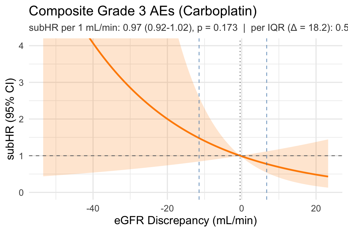
10.8 Composite Grade 3 AEs

Code
plot_subhr_linear_egfrdisc("cmp_time_grade_3_aes", "cmp_status_grade_3_aes",
                           c("pre_HGB_45days", "pre_PLT_45days"), "Composite Grade 3 AEs (Carboplatin)")

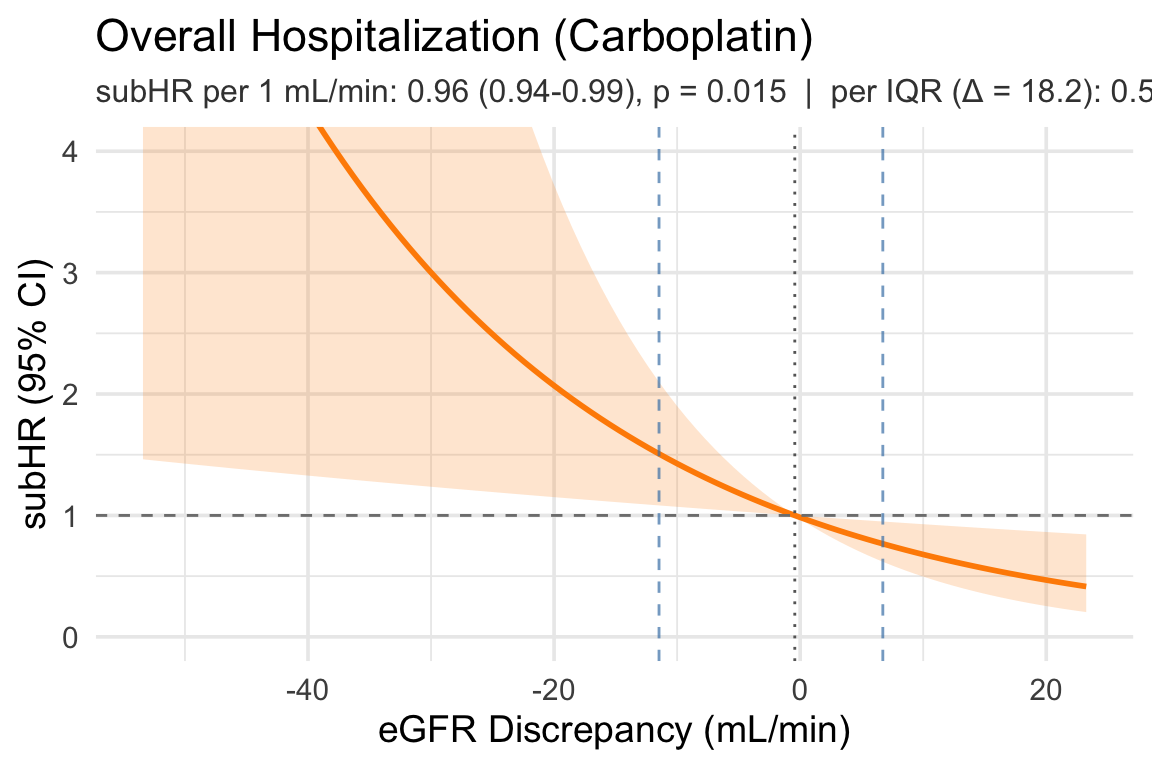
10.9 Overall Hospitalization

Code
plot_subhr_linear_egfrdisc("cmp_time_any_hosp", "cmp_status_any_hosp",
                           NULL, "Overall Hospitalization (Carboplatin)")

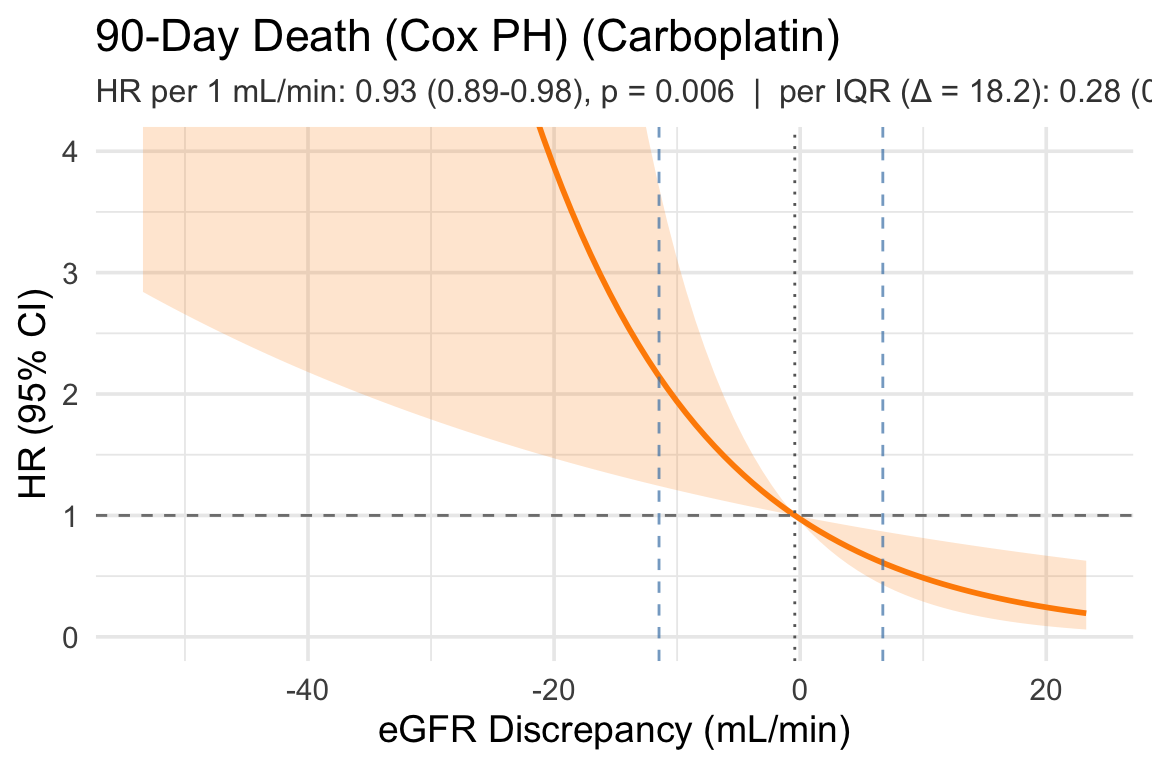
10.11 90-Day Death (Cox PH)

Code
plot_cox_linear_egfrdisc("time_to_death_90", "death_90",
                         NULL, "90-Day Death (Cox PH) (Carboplatin)")

11 Linear subHR Curves — Dose Discrepancy (raw scale) (Carboplatin)

Code
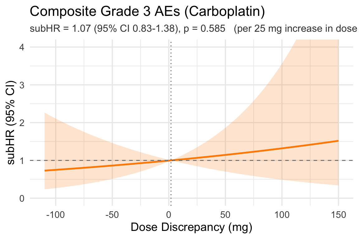
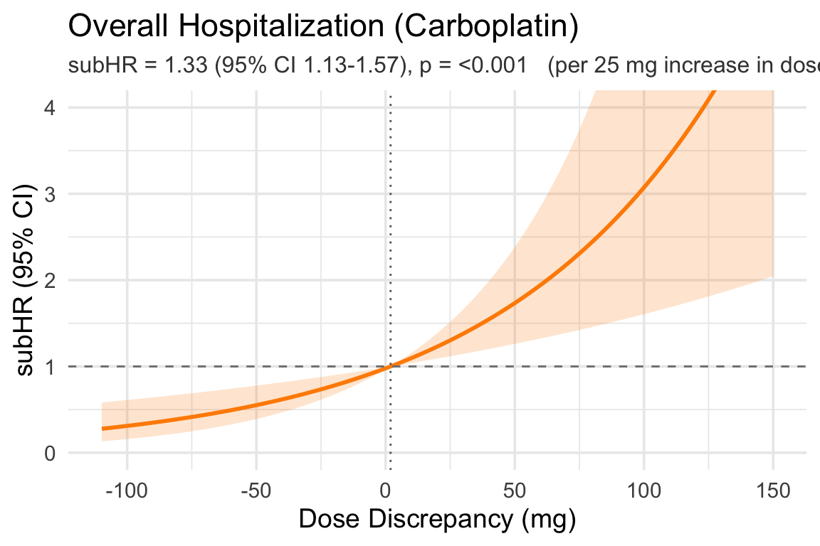
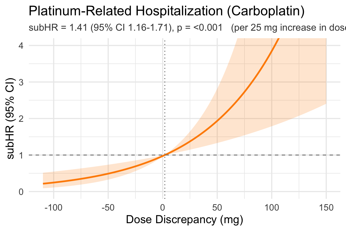
plot_subhr_linear <- function(time_var, status_var, extra_adj = NULL,
                              outcome_label) {
  base_adj <- c("age", "sex", "ecog_score", "ici", "cockcroft")
  keep <- c("dose_discrepancy", time_var, status_var, base_adj, extra_adj)
  d <- dat %>% dplyr::select(all_of(keep)) %>% tidyr::drop_na()

  adj_df <- d[, c(base_adj, extra_adj), drop = FALSE]
  X_adj <- model.matrix(~ ., data = adj_df)[, -1, drop = FALSE]
  X <- cbind(dose_discrepancy = d$dose_discrepancy, X_adj)

  stat_num <- suppressWarnings(as.integer(as.character(d[[status_var]])))
  time_num <- as.numeric(d[[time_var]])

  fit <- tryCatch(
    cmprsk::crr(ftime = time_num, fstatus = stat_num,
                cov1 = X, failcode = 1),
    error = function(e) NULL
  )
  if (is.null(fit)) return(.plot_failed(outcome_label))

  beta   <- fit$coef[1]
  V_beta <- fit$var[1, 1]
  subtitle_str <- .hr_subtitle(beta, V_beta, scale = 25,
                               hr_type = "subHR",
                               unit_label = "per 25 mg increase in dose discrepancy")

  ref_x  <- median(d$dose_discrepancy, na.rm = TRUE)
  grid_x <- seq(quantile(d$dose_discrepancy, 0.025, na.rm = TRUE),
                quantile(d$dose_discrepancy, 0.975, na.rm = TRUE),
                length.out = 100)

  log_hr <- beta * (grid_x - ref_x)
  se     <- sqrt((grid_x - ref_x)^2 * V_beta)

  df_plot <- tibble(
    x     = grid_x,
    subhr = exp(log_hr),
    lcl   = exp(log_hr - 1.96 * se),
    ucl   = exp(log_hr + 1.96 * se)
  )

  ggplot(df_plot, aes(x = x, y = subhr)) +
    geom_ribbon(aes(ymin = lcl, ymax = ucl), alpha = 0.2, fill = "darkorange") +
    geom_line(color = "darkorange", linewidth = 1) +
    geom_hline(yintercept = 1, linetype = "dashed", color = "grey50") +
    geom_vline(xintercept = ref_x, linetype = "dotted", color = "grey40") +
    labs(x = "Dose Discrepancy (mg)",
         y = "subHR (95% CI)",
         title = outcome_label,
         subtitle = subtitle_str) +
    coord_cartesian(ylim = c(0, 4)) +
    theme_minimal(base_size = 14) +
    theme(plot.subtitle = element_text(size = 12, color = "grey25")) -> p
  .save_plot_pptx(p)
  p
}
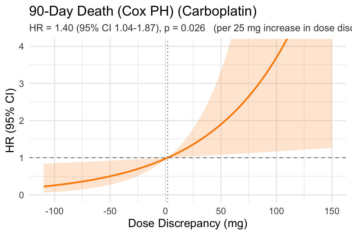
plot_cox_linear <- function(time_var, status_var, extra_adj = NULL,
                            outcome_label) {
  base_adj <- c("age", "sex", "ecog_score", "ici", "cockcroft")
  keep <- c("dose_discrepancy", time_var, status_var, base_adj, extra_adj)
  d <- dat %>% dplyr::select(all_of(keep)) %>% tidyr::drop_na()

  fmla <- as.formula(paste0(
    "Surv(", time_var, ", ", status_var, ") ~ dose_discrepancy + ",
    paste(c(base_adj, extra_adj), collapse = " + ")
  ))
  fit <- tryCatch(survival::coxph(fmla, data = d), error = function(e) NULL)
  if (is.null(fit)) return(.plot_failed(outcome_label))

  beta   <- coef(fit)["dose_discrepancy"]
  V_beta <- vcov(fit)["dose_discrepancy", "dose_discrepancy"]
  subtitle_str <- .hr_subtitle(beta, V_beta, scale = 25,
                               hr_type = "HR",
                               unit_label = "per 25 mg increase in dose discrepancy (Cox PH)")

  ref_x  <- median(d$dose_discrepancy, na.rm = TRUE)
  grid_x <- seq(quantile(d$dose_discrepancy, 0.025, na.rm = TRUE),
                quantile(d$dose_discrepancy, 0.975, na.rm = TRUE),
                length.out = 100)

  log_hr <- beta * (grid_x - ref_x)
  se     <- sqrt((grid_x - ref_x)^2 * V_beta)

  df_plot <- tibble(
    x   = grid_x,
    hr  = exp(log_hr),
    lcl = exp(log_hr - 1.96 * se),
    ucl = exp(log_hr + 1.96 * se)
  )

  ggplot(df_plot, aes(x = x, y = hr)) +
    geom_ribbon(aes(ymin = lcl, ymax = ucl), alpha = 0.2, fill = "darkorange") +
    geom_line(color = "darkorange", linewidth = 1) +
    geom_hline(yintercept = 1, linetype = "dashed", color = "grey50") +
    geom_vline(xintercept = ref_x, linetype = "dotted", color = "grey40") +
    labs(x = "Dose Discrepancy (mg)",
         y = "HR (95% CI)",
         title = outcome_label,
         subtitle = subtitle_str) +
    coord_cartesian(ylim = c(0, 4)) +
    theme_minimal(base_size = 14) +
    theme(plot.subtitle = element_text(size = 12, color = "grey25")) -> p
  .save_plot_pptx(p)
  p
}
11.1 Anemia Grade 2

Code
plot_subhr_linear("cmp_time_anemia_2", "cmp_status_anemia_2",
                  "pre_HGB_45days", "Anemia Grade 2 (Carboplatin)")

11.2 Anemia Grade 3

Code
plot_subhr_linear("cmp_time_anemia_3", "cmp_status_anemia_3",
                  "pre_HGB_45days", "Anemia Grade 3 (Carboplatin)")

11.3 Thrombocytopenia Grade 2

Code
plot_subhr_linear("cmp_time_throm_2", "cmp_status_throm_2",
                  "pre_PLT_45days", "Thrombocytopenia Grade 2 (Carboplatin)")

11.4 Thrombocytopenia Grade 3

Code
plot_subhr_linear("cmp_time_throm_3", "cmp_status_throm_3",
                  "pre_PLT_45days", "Thrombocytopenia Grade 3 (Carboplatin)")

11.5 AKI Grade 2

Code
plot_subhr_linear("cmp_time_aki_2", "cmp_status_aki_2",
                  NULL, "AKI Grade 2 (Carboplatin)")

11.6 AKI (KDIGO)

Code
plot_subhr_linear("cmp_time_aki_kdigo", "cmp_status_aki_kdigo",
                  NULL, "AKI (KDIGO) (Carboplatin)")

11.7 Composite Grade 2 AEs

Code
plot_subhr_linear("cmp_time_grade_2_aes", "cmp_status_grade_2_aes",
                  c("pre_HGB_45days", "pre_PLT_45days"), "Composite Grade 2 AEs (Carboplatin)")

11.8 Composite Grade 3 AEs

Code
plot_subhr_linear("cmp_time_grade_3_aes", "cmp_status_grade_3_aes",
                  c("pre_HGB_45days", "pre_PLT_45days"), "Composite Grade 3 AEs (Carboplatin)")

11.9 Overall Hospitalization

Code
plot_subhr_linear("cmp_time_any_hosp", "cmp_status_any_hosp",
                  NULL, "Overall Hospitalization (Carboplatin)")

11.11 90-Day Death (Cox PH)

Code
plot_cox_linear("time_to_death_90", "death_90",
                NULL, "90-Day Death (Cox PH) (Carboplatin)")

12 Linear subHR Curves — Hospitalization by Reason (Carboplatin)

13.1 Nausea/Vomiting/GI

Code
plot_subhr_linear_ratio("cmp_time_hosp_1", "cmp_status_hosp_1",
                        NULL, "Nausea/Vomiting/GI (Carboplatin)")

13.2 Failure to Thrive/Fatigue/Dehydration

Code
plot_subhr_linear_ratio("cmp_time_hosp_2", "cmp_status_hosp_2",
                        NULL, "Failure to Thrive/Fatigue/Dehydration (Carboplatin)")

13.3 AKI

Code
plot_subhr_linear_ratio("cmp_time_hosp_3", "cmp_status_hosp_3",
                        NULL, "AKI (Carboplatin)")

13.4 Electrolyte Abnormalities

Code
plot_subhr_linear_ratio("cmp_time_hosp_4", "cmp_status_hosp_4",
                        NULL, "Electrolyte Abnormalities (Carboplatin)")

13.5 Cytopenia

Code
plot_subhr_linear_ratio("cmp_time_hosp_5", "cmp_status_hosp_5",
                        NULL, "Cytopenia (Carboplatin)")

13.6 Febrile Neutropenia

Code
plot_subhr_linear_ratio("cmp_time_hosp_6", "cmp_status_hosp_6",
                        NULL, "Febrile Neutropenia (Carboplatin)")

13.7 Infection/Sepsis

Code
plot_subhr_linear_ratio("cmp_time_hosp_7", "cmp_status_hosp_7",
                        NULL, "Infection/Sepsis (Carboplatin)")

13.8 Cancer Progression

Code
plot_subhr_linear_ratio("cmp_time_hosp_8", "cmp_status_hosp_8",
                        NULL, "Cancer Progression (Carboplatin)")

13.10 Planned Surgery/Port

Code
plot_subhr_linear_ratio("cmp_time_hosp_10", "cmp_status_hosp_10",
                        NULL, "Planned Surgery/Port (Carboplatin)")

13 Scatter Plots — Dose Discrepancy vs eGFR (Carboplatin)

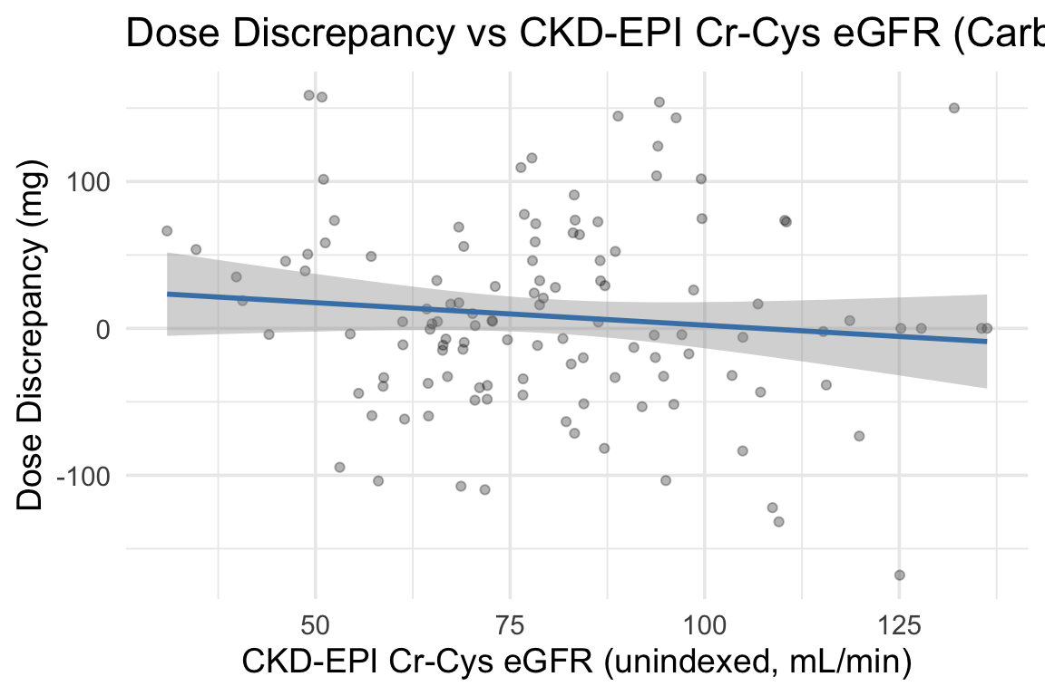
13.1 Dose Discrepancy vs CKD-EPI Cr-Cys (unindexed)

Code
ggplot(dat %>% filter(!is.na(dose_discrepancy)),
       aes(x = ckd_epi_gfr_cre_cys_unindex, y = dose_discrepancy)) +
  geom_point(alpha = 0.3) +
  geom_smooth(method = "lm", se = TRUE, color = "steelblue") +
  labs(x = "CKD-EPI Cr-Cys eGFR (unindexed, mL/min)",
       y = "Dose Discrepancy (mg)",
       title = "Dose Discrepancy vs CKD-EPI Cr-Cys eGFR (Carboplatin)") +
  theme_minimal(base_size = 14) -> p
.save_plot_pptx(p)
p

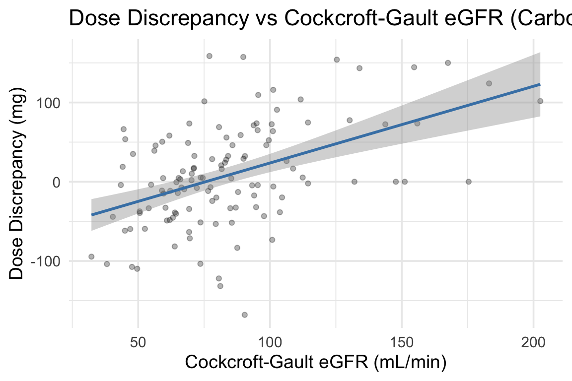
13.2 Dose Discrepancy vs Cockcroft-Gault

Code
ggplot(dat %>% filter(!is.na(dose_discrepancy)),
       aes(x = cockcroft, y = dose_discrepancy)) +
  geom_point(alpha = 0.3) +
  geom_smooth(method = "lm", se = TRUE, color = "steelblue") +
  labs(x = "Cockcroft-Gault eGFR (mL/min)",
       y = "Dose Discrepancy (mg)",
       title = "Dose Discrepancy vs Cockcroft-Gault eGFR (Carboplatin)") +
  theme_minimal(base_size = 14) -> p
.save_plot_pptx(p)
p

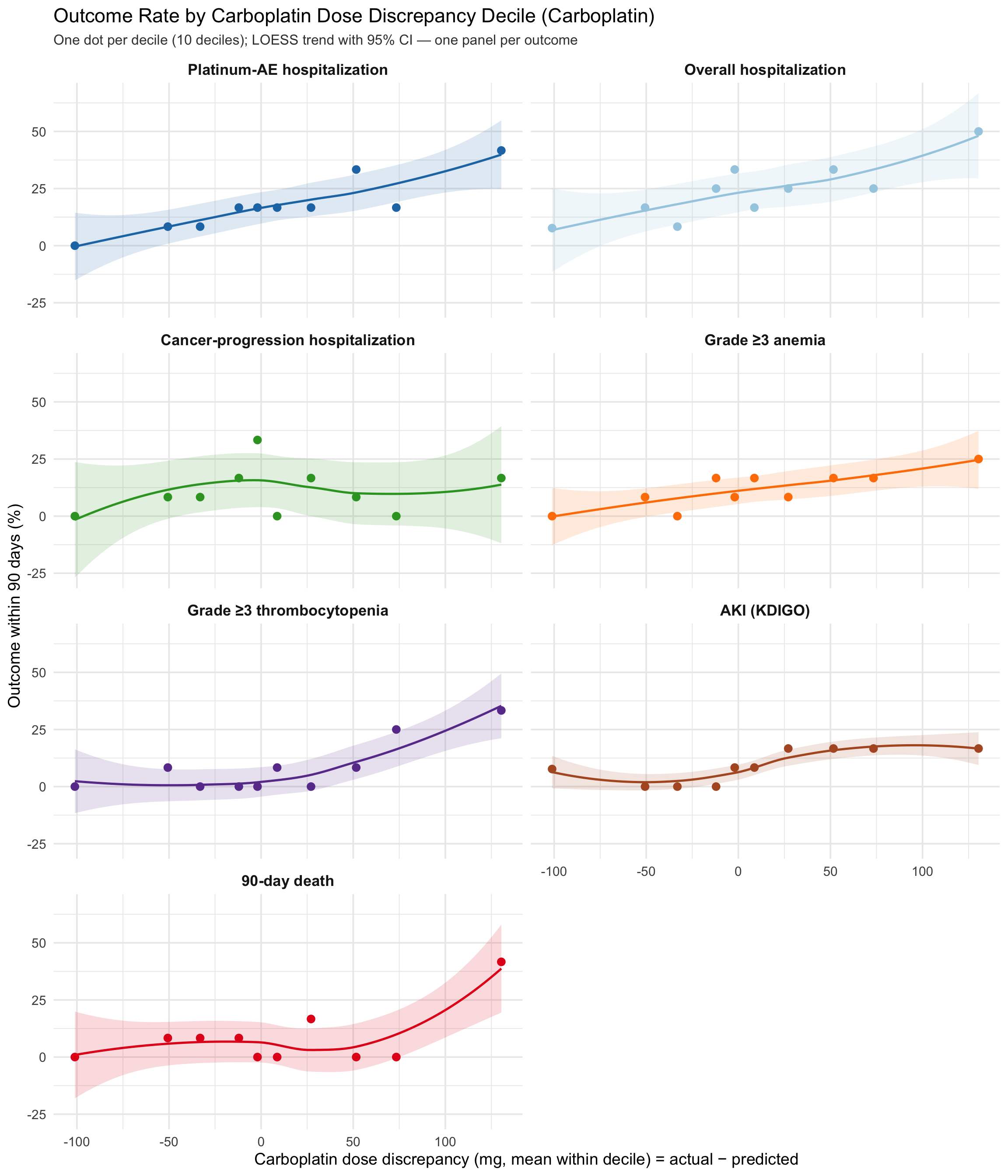
14 Loess — Outcome % by Dose Discrepancy Decile (Carboplatin)

Patients are split into deciles of carboplatin dose discrepancy (actual − predicted dose, mg; 10 equal-sized groups). Each dot is one decile: the x-position is the decile’s mean dose discrepancy and the y-position is the observed percentage of patients in that decile who had the outcome within 90 days. A LOESS curve is overlaid to show the trend. Seven outcomes are shown, grouped as hospitalization (platinum-AE, overall, cancer-progression), grade ≥ 3 toxicity (anemia, thrombocytopenia, AKI by KDIGO) and 90-day death.

Code
.OUTCOME_LEVELS <- c(
  "Platinum-AE hospitalization",
  "Overall hospitalization",
  "Cancer-progression hospitalization",
  "Grade ≥3 anemia",
  "Grade ≥3 thrombocytopenia",
  "AKI (KDIGO)",
  "90-day death")

.OUTCOME_COLS <- c(
  "Platinum-AE hospitalization"        = "#1F78B4",  # blue
  "Overall hospitalization"            = "#A6CEE3",  # light blue
  "Cancer-progression hospitalization" = "#33A02C",  # green
  "Grade ≥3 anemia"                    = "#FF7F00",  # orange
  "Grade ≥3 thrombocytopenia"          = "#6A3D9A",  # purple
  "AKI (KDIGO)"                        = "#B15928",  # brown
  "90-day death"                       = "#E31A1C")  # red

# 1 = event within 90 days, for each competing-risk status variable.
.evt <- function(x) as.integer(suppressWarnings(as.integer(as.character(x))) == 1)

loess_df <- dat %>%
  filter(!is.na(dose_discrepancy)) %>%
  mutate(
    plat_ae     = .evt(cmp_status_side_effect),
    any_hosp    = .evt(cmp_status_any_hosp),
    cancer_prog = .evt(cmp_status_hosp_8),
    anemia3     = .evt(cmp_status_anemia_3),
    throm3      = .evt(cmp_status_throm_3),
    aki_kdigo   = .evt(cmp_status_aki_kdigo),
    death       = .evt(death_90),
    # 10 equal-frequency deciles of dose discrepancy
    decile = dplyr::ntile(dose_discrepancy, 10)
  )

decile_summary <- loess_df %>%
  group_by(decile) %>%
  summarise(
    dd_mean = mean(dose_discrepancy, na.rm = TRUE),
    n       = dplyr::n(),
    `Platinum-AE hospitalization`        = 100 * mean(plat_ae,     na.rm = TRUE),
    `Overall hospitalization`            = 100 * mean(any_hosp,    na.rm = TRUE),
    `Cancer-progression hospitalization` = 100 * mean(cancer_prog, na.rm = TRUE),
    `Grade ≥3 anemia`                    = 100 * mean(anemia3,     na.rm = TRUE),
    `Grade ≥3 thrombocytopenia`          = 100 * mean(throm3,      na.rm = TRUE),
    `AKI (KDIGO)`                        = 100 * mean(aki_kdigo,   na.rm = TRUE),
    `90-day death`                       = 100 * mean(death,       na.rm = TRUE),
    .groups = "drop"
  ) %>%
  tidyr::pivot_longer(
    cols = all_of(.OUTCOME_LEVELS),
    names_to = "outcome", values_to = "pct"
  ) %>%
  mutate(outcome = factor(outcome, levels = .OUTCOME_LEVELS))

ggplot(decile_summary, aes(x = dd_mean, y = pct, color = outcome, fill = outcome)) +
  geom_smooth(method = "loess", se = TRUE, alpha = 0.15, linewidth = 0.9,
              span = 1) +
  geom_point(size = 2.8) +
  facet_wrap(~ outcome, ncol = 2, scales = "fixed") +
  scale_color_manual(values = .OUTCOME_COLS, guide = "none") +
  scale_fill_manual(values = .OUTCOME_COLS, guide = "none") +
  labs(title = "Outcome Rate by Carboplatin Dose Discrepancy Decile (Carboplatin)",
       subtitle = "One dot per decile (10 deciles); LOESS trend with 95% CI — one panel per outcome",
       x = "Carboplatin dose discrepancy (mg, mean within decile) = actual − predicted",
       y = "Outcome within 90 days (%)") +
  theme_minimal(base_size = 14) +
  theme(plot.subtitle = element_text(size = 12, color = "grey25"),
        strip.text = element_text(size = 13, face = "bold")) -> p
.save_plot_pptx(p)
p

15 Adjusted CIF — Dose Discrepancy >= +25 mg (Carboplatin)

Standardized cumulative incidence functions for each competing-risk outcome, contrasting patients with dose_discrepancy >= 25 (red) against those with dose_discrepancy < 25 (blue). The Fine-Gray model is fit with the binary exposure plus the same adjuster set used in Section 7. Curves are adjusted (standardized) via g-computation: for every patient, predict CIF under exposure = 1 and under exposure = 0, then average the two CIF curves over the cohort. Y-axis is cumulative incidence, x-axis is days from baseline.

90-day death (Section 15.11) is modelled with Cox PH instead of Fine-Gray (no competing event), and the standardized cumulative-incidence-of-death curve is 1 − S(t|Xᵢ) averaged across the cohort.

Code
adj_cif <- function(time_var, status_var, extra_pre = NULL, label) {
  base_adj <- c("age", "sex", "ecog_score", "ici", "cockcroft")
  vars <- c("dose_discrep_ge25", base_adj, extra_pre)
  d <- dat %>%
    dplyr::select(all_of(c(time_var, status_var, vars))) %>%
    tidyr::drop_na()

  fmla <- as.formula(paste("~",
            paste(c("dose_discrep_ge25", base_adj, extra_pre), collapse = " + ")))
  X_full <- model.matrix(fmla, data = d)[, -1, drop = FALSE]

  stat_num <- suppressWarnings(as.integer(as.character(d[[status_var]])))
  time_num <- as.numeric(d[[time_var]])

  fit <- tryCatch(
    cmprsk::crr(ftime = time_num, fstatus = stat_num,
                cov1 = X_full, failcode = 1),
    error = function(e) NULL
  )
  if (is.null(fit)) return(.plot_failed(label))

  # subHR (95% CI) for the binary exposure, extracted from the same FG fit
  # dose_discrep_ge25 is the first column of cov1 (entered first in the formula)
  beta_e <- unname(fit$coef[1])
  se_e   <- sqrt(fit$var[1, 1])
  hr     <- exp(beta_e)
  lcl    <- exp(beta_e - 1.96 * se_e)
  ucl    <- exp(beta_e + 1.96 * se_e)
  pval   <- 2 * (1 - pnorm(abs(beta_e / se_e)))
  p_str  <- ifelse(pval < 0.001, "<0.001", sprintf("%.3f", pval))
  subtitle_str <- sprintf(
    "Discrep >= +25 vs <+25: subHR = %.2f (95%% CI %.2f-%.2f), p = %s",
    hr, lcl, ucl, p_str
  )

  X0 <- X_full; X0[, "dose_discrep_ge25"] <- 0
  X1 <- X_full; X1[, "dose_discrep_ge25"] <- 1

  pred0 <- predict(fit, X0)
  pred1 <- predict(fit, X1)

  times <- pred0[, 1]
  cif0  <- rowMeans(pred0[, -1, drop = FALSE])
  cif1  <- rowMeans(pred1[, -1, drop = FALSE])

  df <- bind_rows(
    tibble(time = times, cif = cif0, group = "Discrep < +25 mg"),
    tibble(time = times, cif = cif1, group = "Discrep >= +25 mg")
  )

  ymax <- max(df$cif, na.rm = TRUE)

  ggplot(df, aes(x = time, y = cif, color = group)) +
    geom_step(linewidth = 1) +
    scale_color_manual(values = c("Discrep < +25 mg"  = "#1F78B4",
                                  "Discrep >= +25 mg" = "#E31A1C")) +
    coord_cartesian(ylim = c(0, max(0.05, ymax * 1.05))) +
    labs(x = "Days from baseline",
         y = "Cumulative incidence",
         color = NULL,
         title = label,
         subtitle = subtitle_str) +
    theme_minimal(base_size = 14) +
    theme(legend.position = "top",
          plot.subtitle = element_text(size = 12, color = "grey25")) -> p
  .save_plot_pptx(p)
  p
}
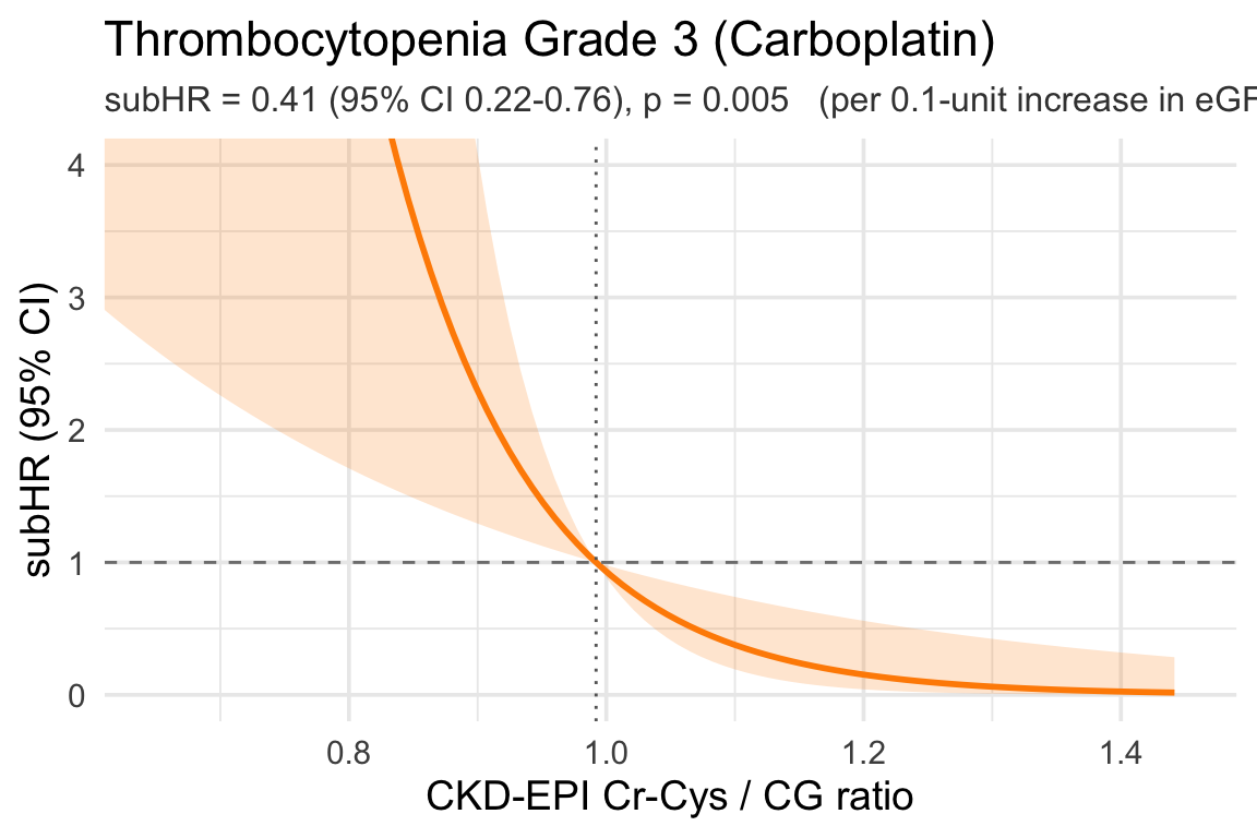
adj_death_curve <- function(time_var = "time_to_death_90",
                            status_var = "death_90", label) {
  base_adj <- c("age", "sex", "ecog_score", "ici", "cockcroft")
  vars <- c("dose_discrep_ge25", base_adj)
  d <- dat %>%
    dplyr::select(all_of(c(time_var, status_var, vars))) %>%
    tidyr::drop_na()

  rhs <- paste(c("dose_discrep_ge25", base_adj), collapse = " + ")
  fmla <- as.formula(sprintf("survival::Surv(%s, %s) ~ %s",
                             time_var, status_var, rhs))
  fit <- tryCatch(survival::coxph(fmla, data = d), error = function(e) NULL)
  if (is.null(fit)) return(.plot_failed(label))

  beta_e <- unname(coef(fit)["dose_discrep_ge25"])
  se_e   <- sqrt(vcov(fit)["dose_discrep_ge25", "dose_discrep_ge25"])
  hr     <- exp(beta_e)
  lcl    <- exp(beta_e - 1.96 * se_e)
  ucl    <- exp(beta_e + 1.96 * se_e)
  pval   <- 2 * (1 - pnorm(abs(beta_e / se_e)))
  p_str  <- ifelse(pval < 0.001, "<0.001", sprintf("%.3f", pval))
  subtitle_str <- sprintf(
    "Discrep >= +25 vs <+25: HR = %.2f (95%% CI %.2f-%.2f), p = %s   (Cox PH)",
    hr, lcl, ucl, p_str
  )

  d0 <- d; d0$dose_discrep_ge25 <- 0
  d1 <- d; d1$dose_discrep_ge25 <- 1

  sf0 <- survival::survfit(fit, newdata = d0)
  sf1 <- survival::survfit(fit, newdata = d1)

  s0 <- if (is.matrix(sf0$surv)) sf0$surv else as.matrix(sf0$surv)
  s1 <- if (is.matrix(sf1$surv)) sf1$surv else as.matrix(sf1$surv)

  cif0 <- 1 - rowMeans(s0)
  cif1 <- 1 - rowMeans(s1)

  df <- bind_rows(
    tibble(time = sf0$time, cif = cif0, group = "Discrep < +25 mg"),
    tibble(time = sf1$time, cif = cif1, group = "Discrep >= +25 mg")
  )

  ymax <- max(df$cif, na.rm = TRUE)

  ggplot(df, aes(x = time, y = cif, color = group)) +
    geom_step(linewidth = 1) +
    scale_color_manual(values = c("Discrep < +25 mg"  = "#1F78B4",
                                  "Discrep >= +25 mg" = "#E31A1C")) +
    coord_cartesian(ylim = c(0, max(0.05, ymax * 1.05))) +
    labs(x = "Days from baseline",
         y = "Cumulative incidence (1 - S)",
         color = NULL,
         title = label,
         subtitle = subtitle_str) +
    theme_minimal(base_size = 14) +
    theme(legend.position = "top",
          plot.subtitle = element_text(size = 12, color = "grey25")) -> p
  .save_plot_pptx(p)
  p
}
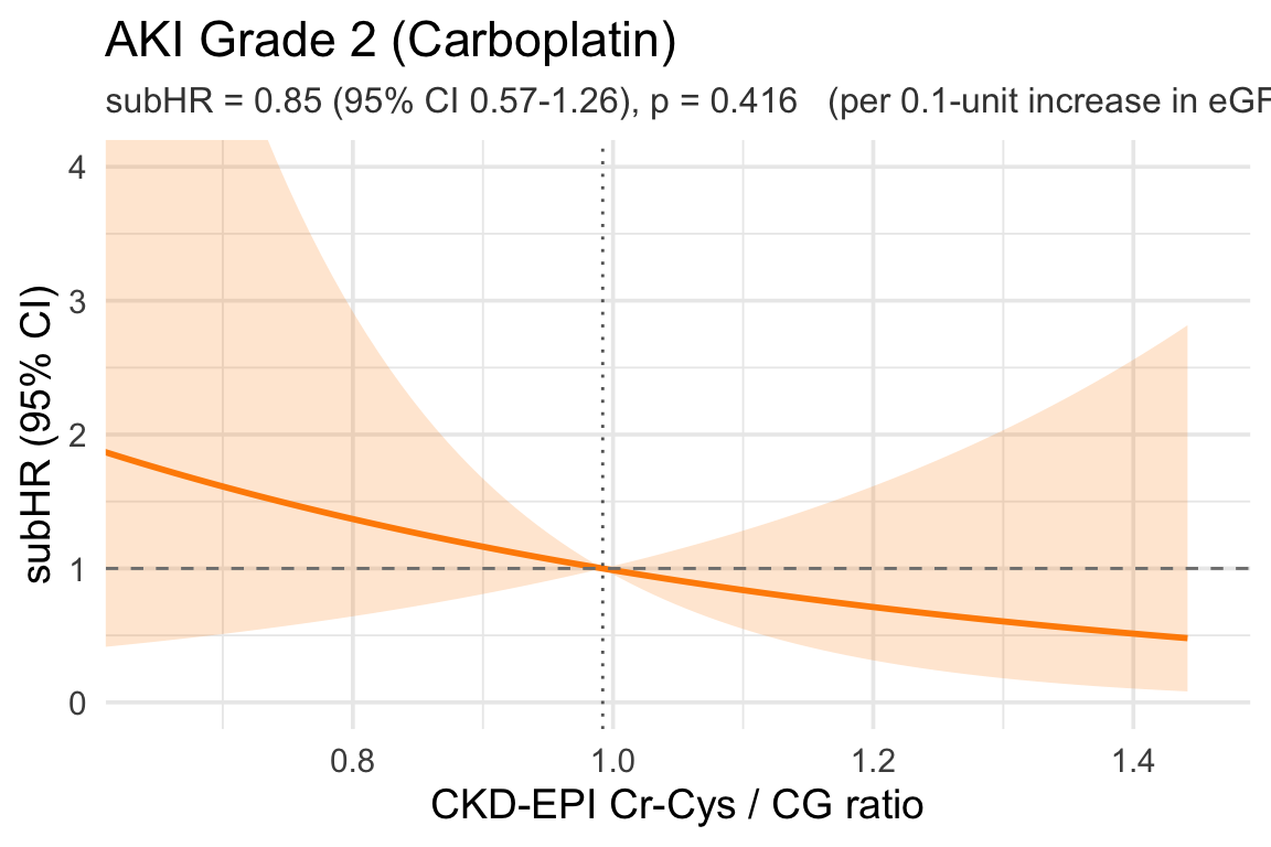
15.1 Anemia Grade 2

Code
adj_cif("cmp_time_anemia_2", "cmp_status_anemia_2",
        "pre_HGB_45days", "Anemia Grade 2")

15.2 Anemia Grade 3

Code
adj_cif("cmp_time_anemia_3", "cmp_status_anemia_3",
        "pre_HGB_45days", "Anemia Grade 3")

15.3 Thrombocytopenia Grade 2

Code
adj_cif("cmp_time_throm_2", "cmp_status_throm_2",
        "pre_PLT_45days", "Thrombocytopenia Grade 2")

15.4 Thrombocytopenia Grade 3

Code
adj_cif("cmp_time_throm_3", "cmp_status_throm_3",
        "pre_PLT_45days", "Thrombocytopenia Grade 3")

15.5 AKI Grade 2

Code
adj_cif("cmp_time_aki_2", "cmp_status_aki_2",
        NULL, "AKI Grade 2")

15.6 AKI (KDIGO)

Code
adj_cif("cmp_time_aki_kdigo", "cmp_status_aki_kdigo",
        NULL, "AKI (KDIGO)")

15.7 Composite Grade 2 AEs

Code
adj_cif("cmp_time_grade_2_aes", "cmp_status_grade_2_aes",
        c("pre_HGB_45days", "pre_PLT_45days"), "Composite Grade 2 AEs")

15.8 Composite Grade 3 AEs

Code
adj_cif("cmp_time_grade_3_aes", "cmp_status_grade_3_aes",
        c("pre_HGB_45days", "pre_PLT_45days"), "Composite Grade 3 AEs")

15.9 Overall Hospitalization

Code
adj_cif("cmp_time_any_hosp", "cmp_status_any_hosp",
        NULL, "Overall Hospitalization")

15.11 90-Day Death (Cox PH)

Code
adj_death_curve("time_to_death_90", "death_90", "90-Day Death")

16 Paper

A total of 44 (36.4%) patients received an excess dose of carboplatin, defined as ≥ 25 mg higher than the dose that would have been predicted using the CKD-EPI eGFRCR-CYS equation adjusted for actual BSA.

(Denominator: 121 carboplatin patients with a computable predicted dose.)

17 Downloadable PowerPoint Plots

Every figure on this page is also saved as an editable PowerPoint slide (vector graphics — text and shapes remain editable in PowerPoint). Click any link below to download the .pptx for that figure.

Code
pptx_files <- list.files(pptx_dir, pattern = "\\.pptx$", full.names = FALSE)
if (length(pptx_files) == 0) {
  cat("*No PowerPoint files were produced during this render.*\n")
} else {
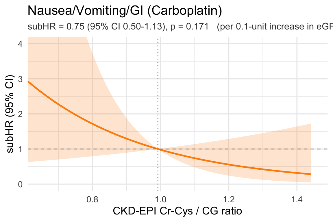
  for (f in sort(pptx_files)) {
    label <- gsub("_", " ", tools::file_path_sans_ext(f))
    cat(sprintf("- [📥 %s](../plots/carbo/%s)\n", label, f))
  }
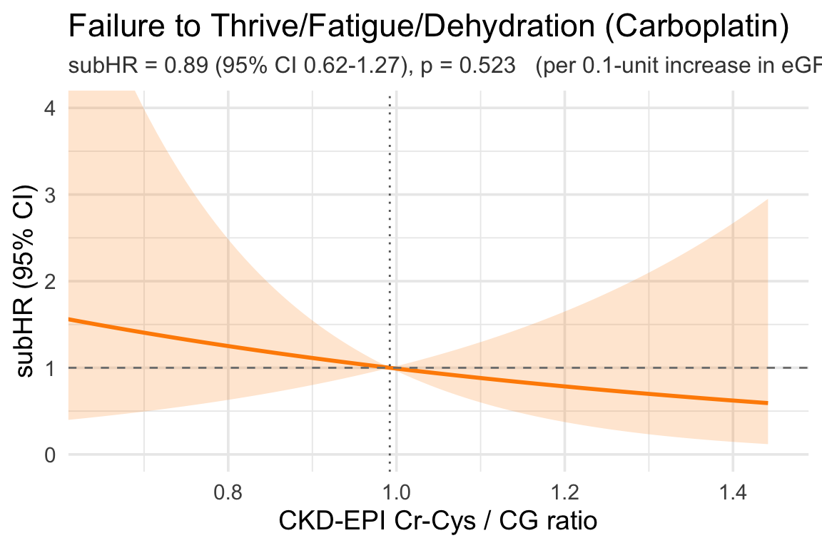
}