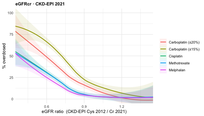
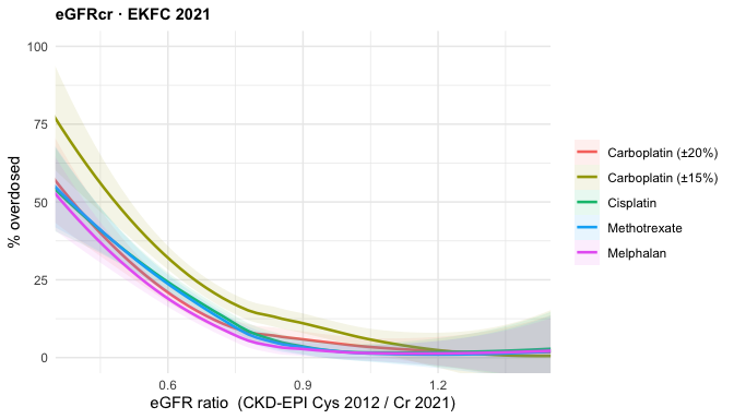
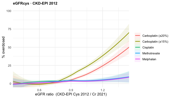
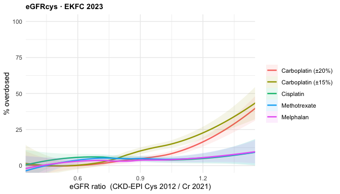
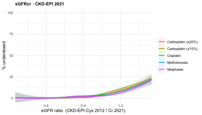
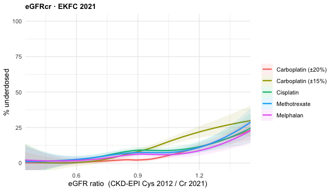
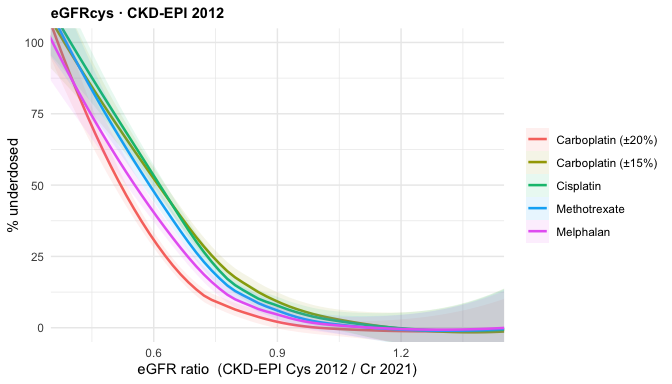
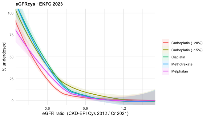
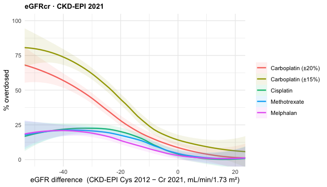
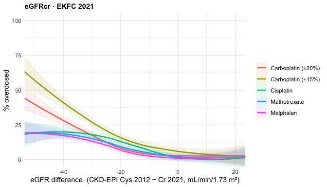
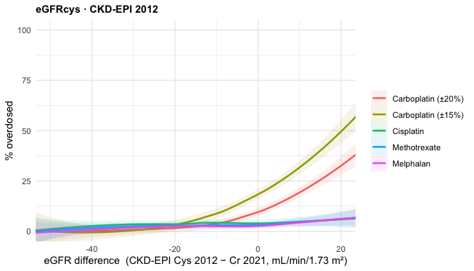
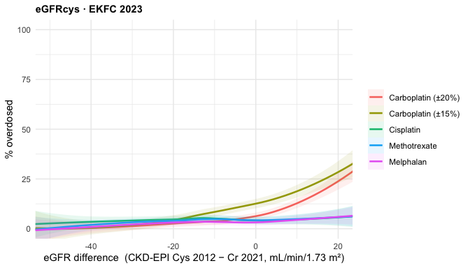
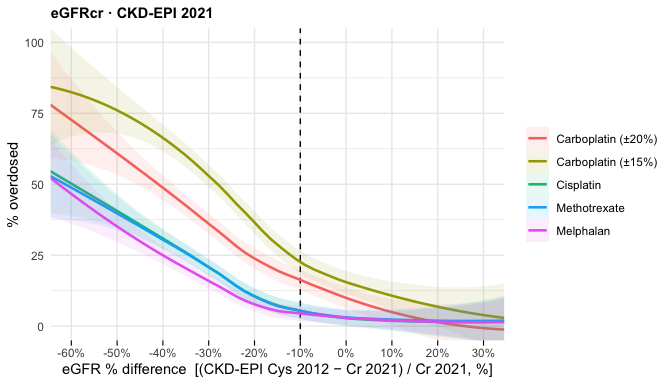
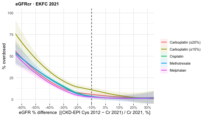
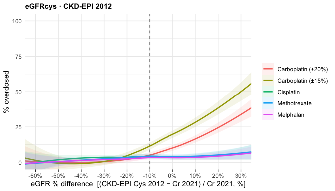
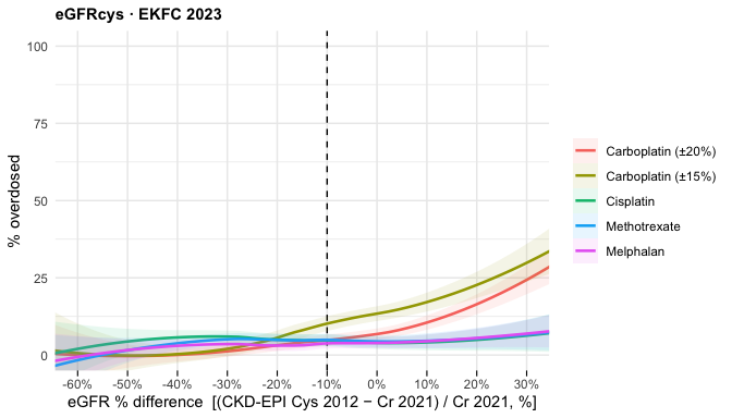
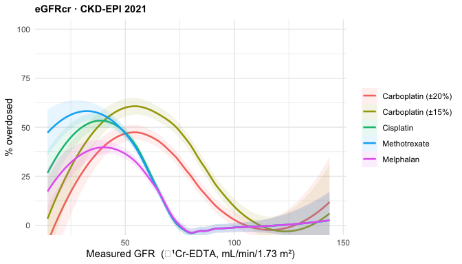
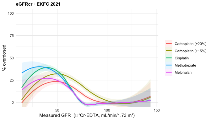
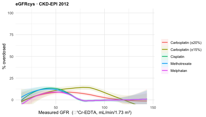
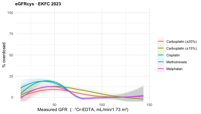
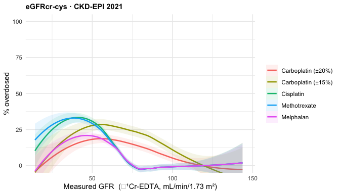
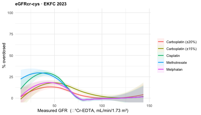
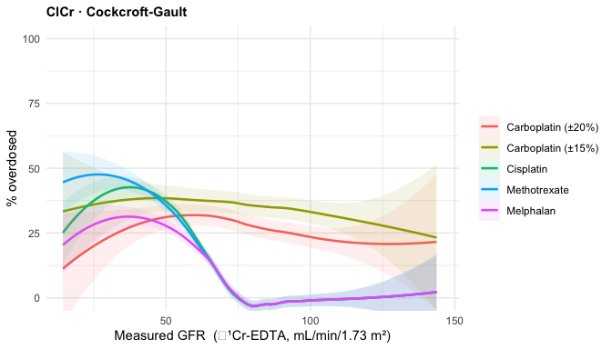
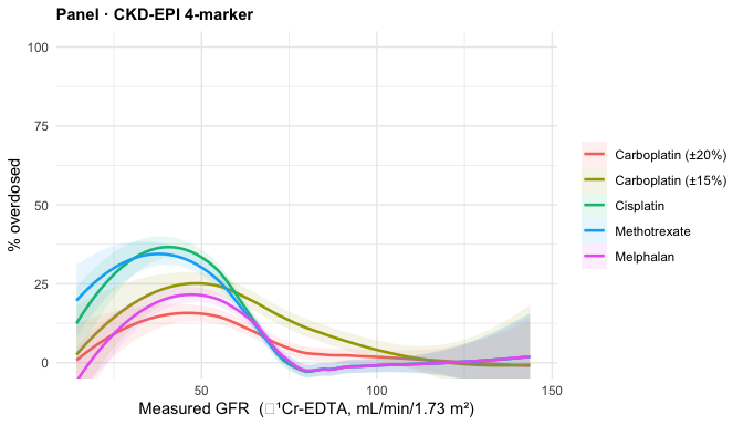
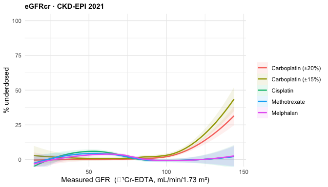
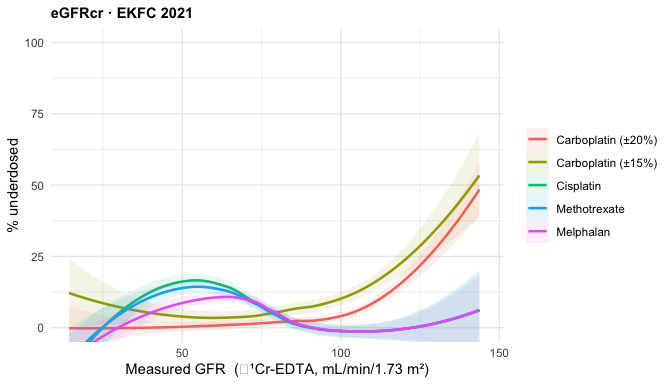
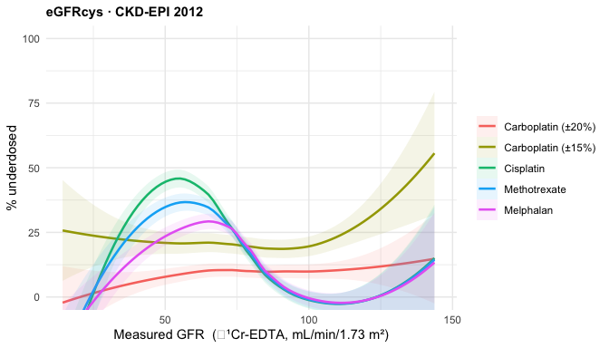
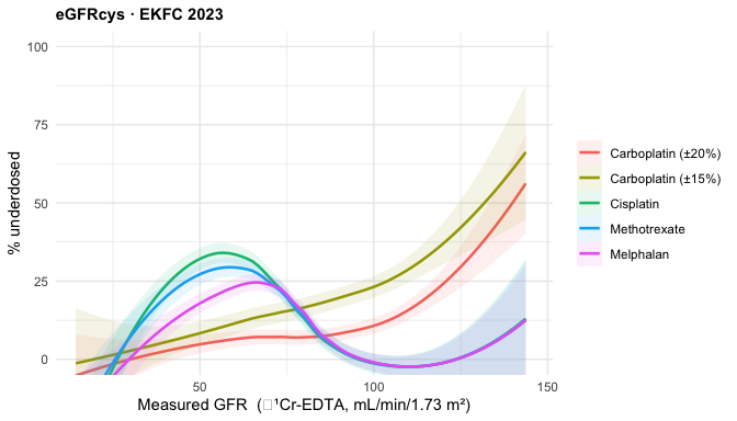
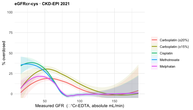
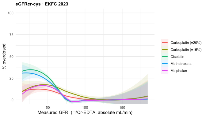
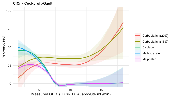
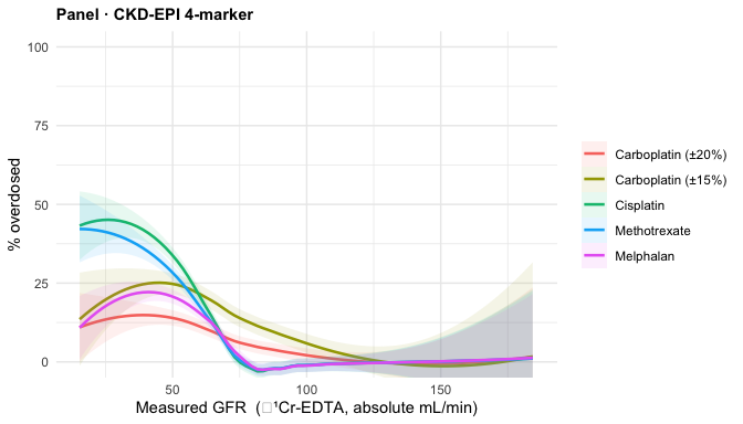
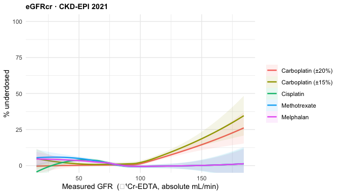
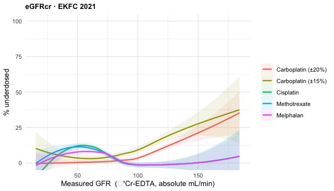
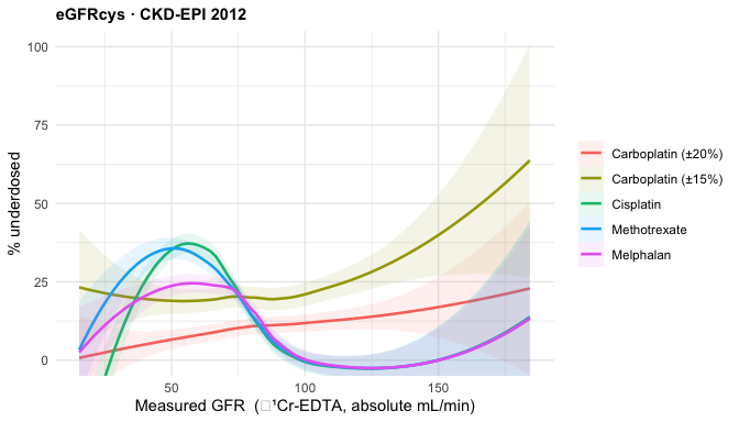
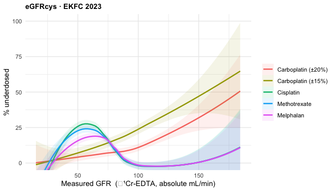
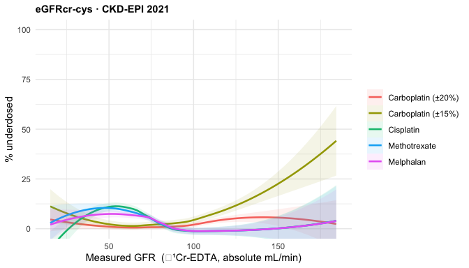
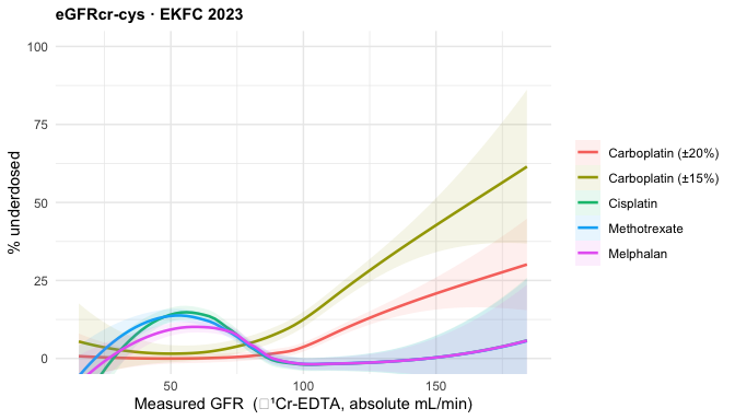
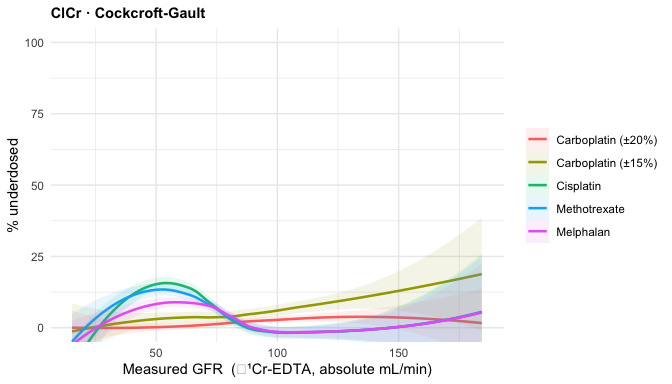
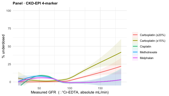
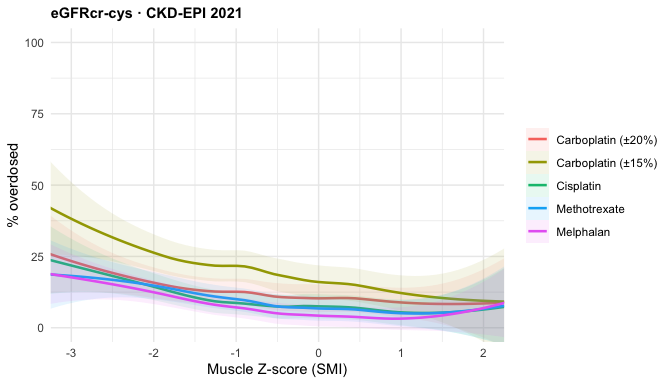
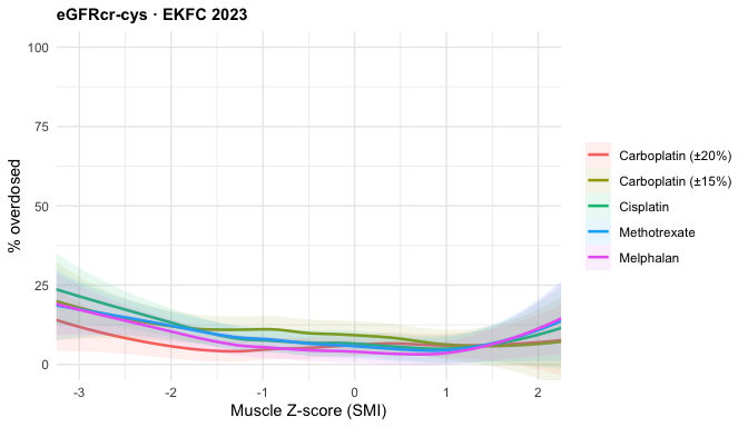
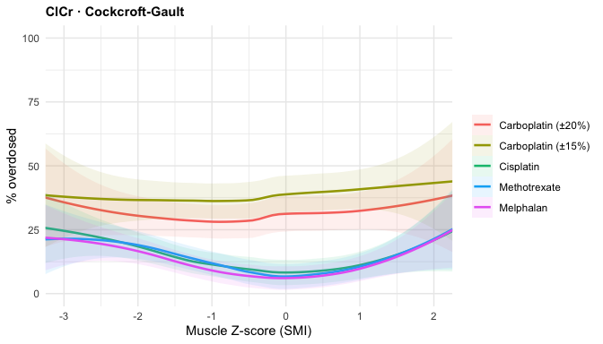
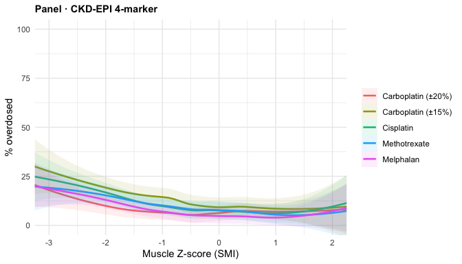
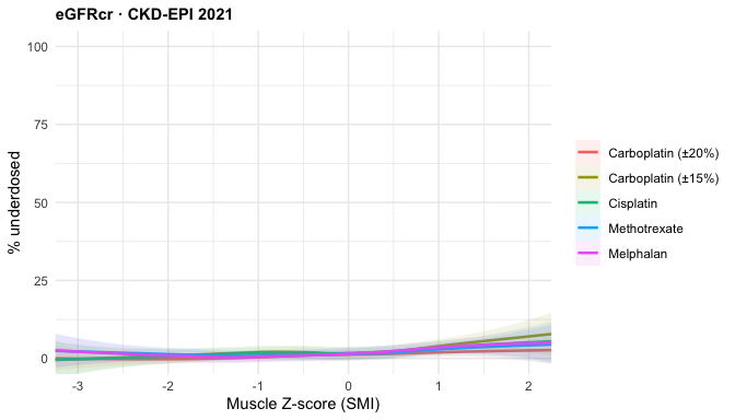
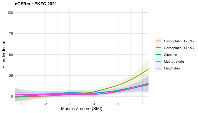
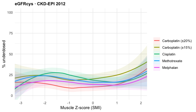
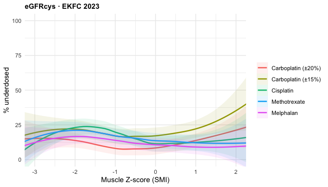
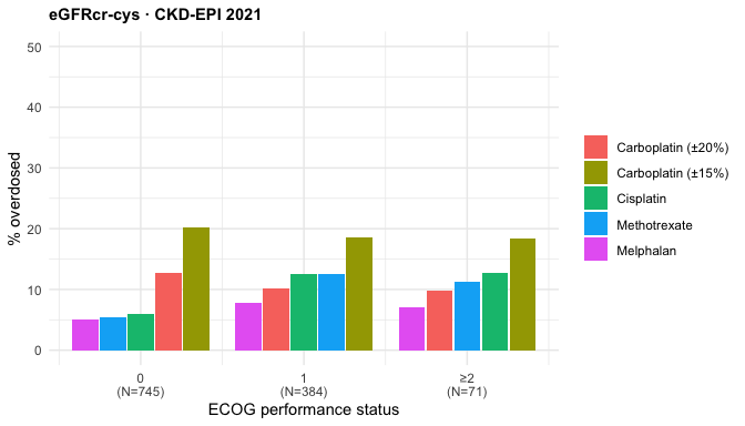
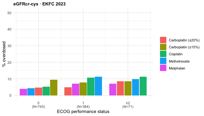
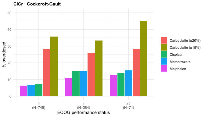
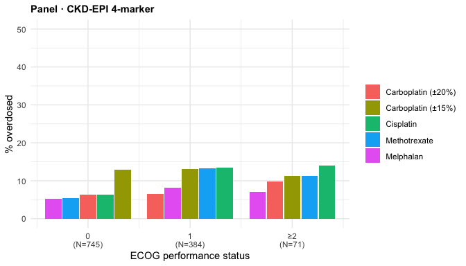
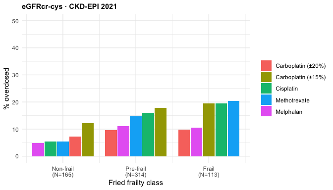
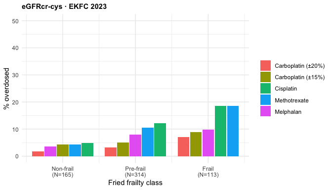
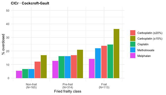
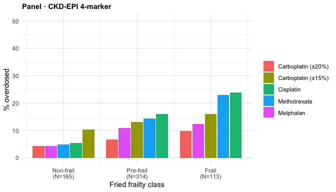
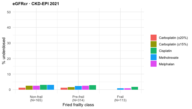
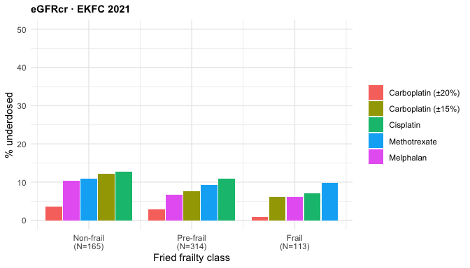
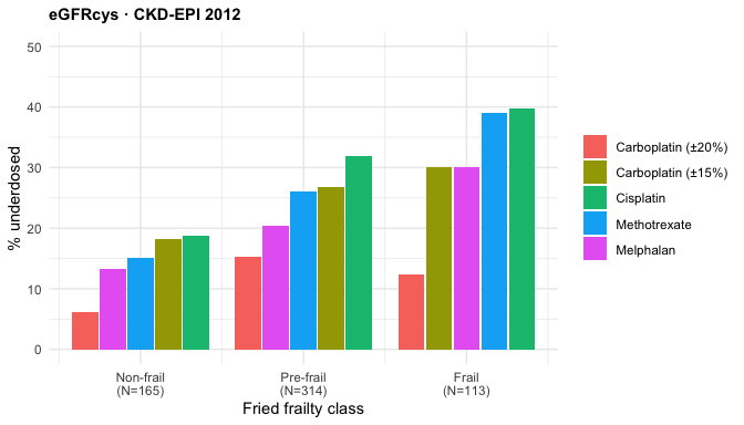
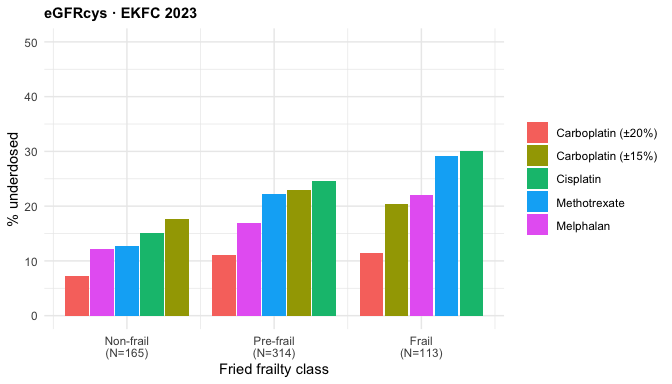
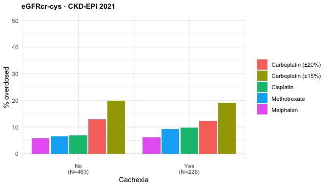
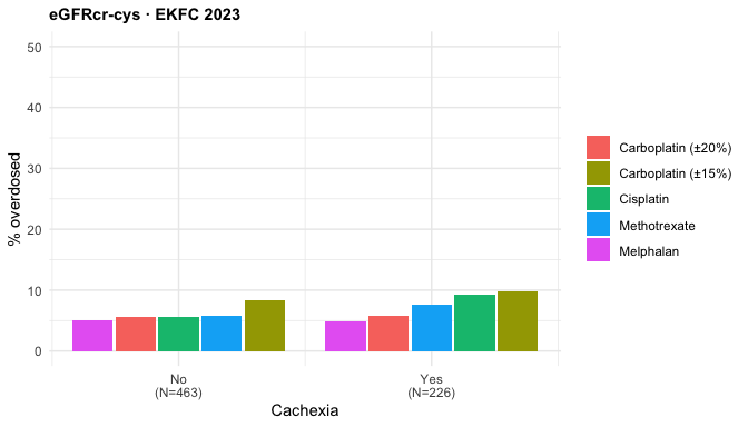
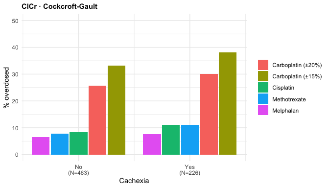
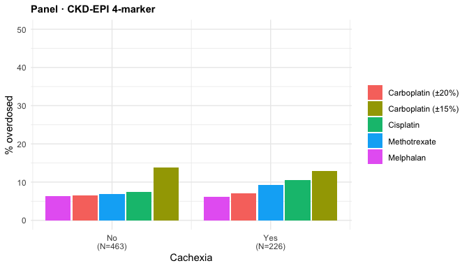
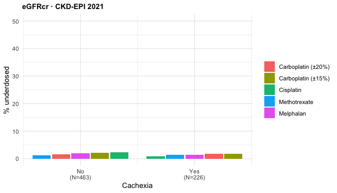
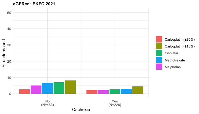
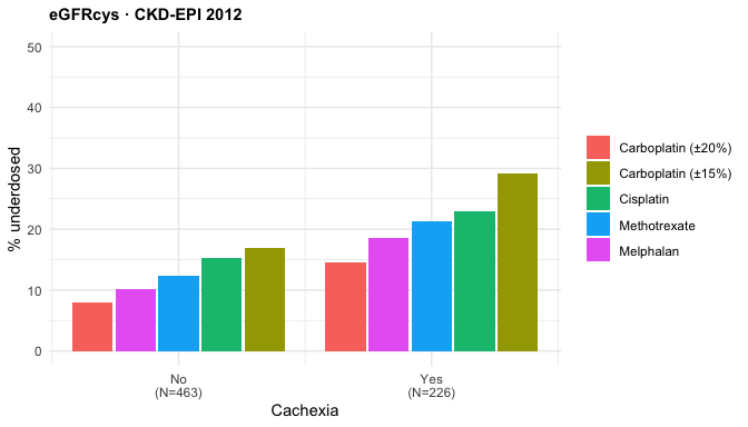
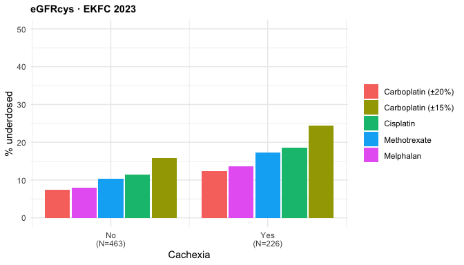
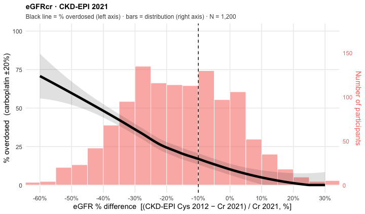
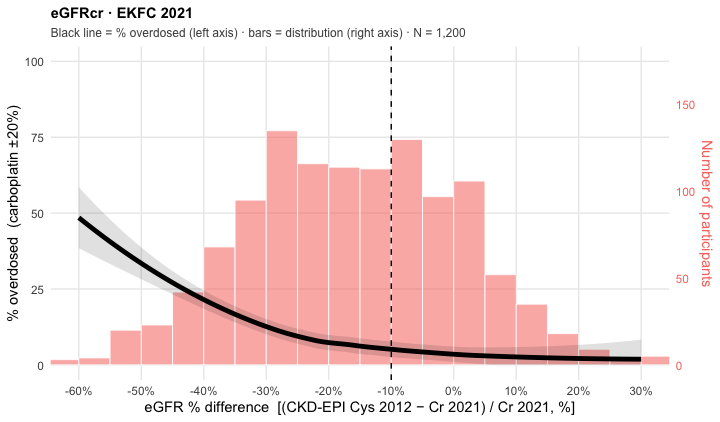
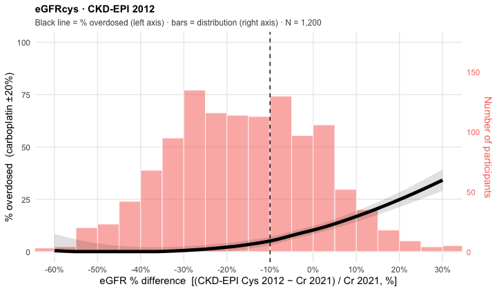
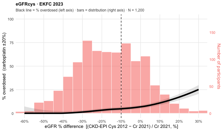
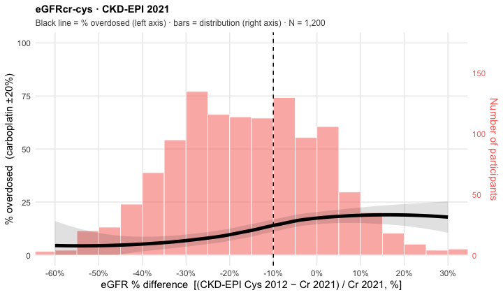
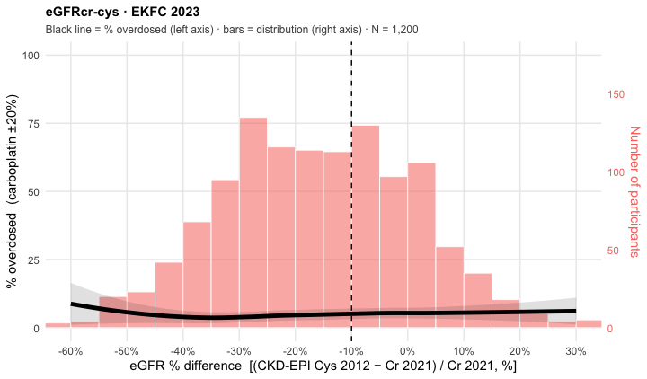
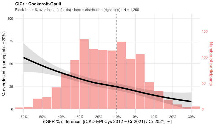
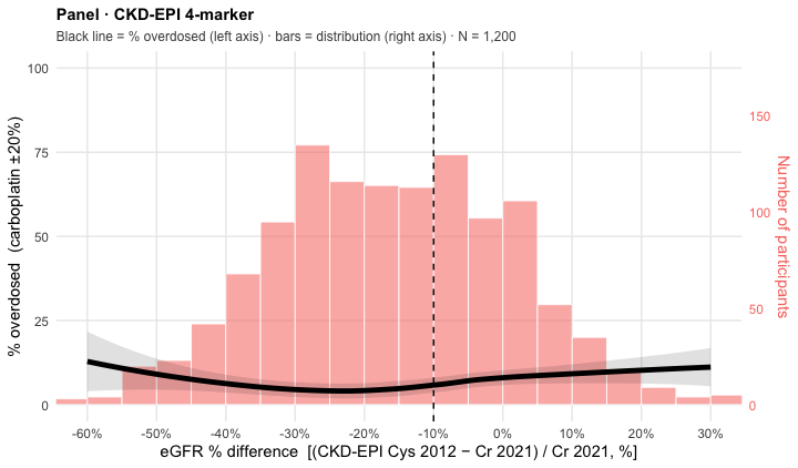
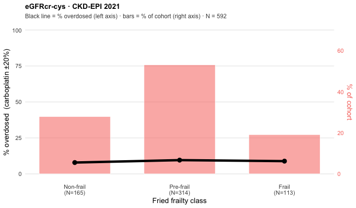
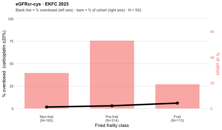
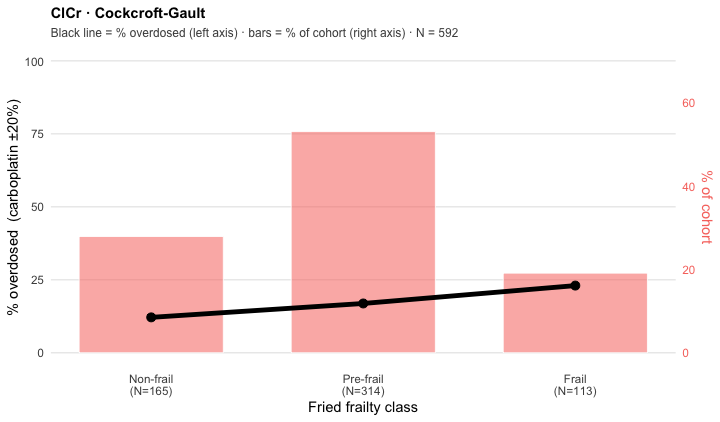
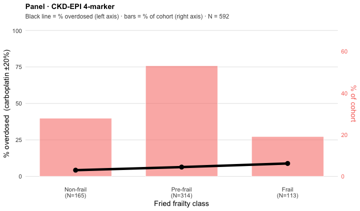
raw <- suppressWarnings(
  readxl::read_excel("Data/OncoGFR1200_MGH_chemo_CJASN.xlsx")
)
dat <- raw %>%
  dplyr::select(-dplyr::any_of(c("...70", "...75"))) %>%
  dplyr::mutate(
    sex     = factor(gender, levels = c(1, 2), labels = c("Male", "Female")),
    bmi_grp = cut(BMI, breaks = c(-Inf, 20, 25, 30, Inf), right = FALSE,
                  labels = c("<20", "20 to <25", "25 to <30", ">=30")),
    # metastasis is complete (0/1) in this dataset — no "Unknown" level.
    met_grp = factor(metastasis, levels = c(0, 1),
                     labels = c("Not metastatic", "Metastatic")),
    age_grp = factor(ifelse(age >= 70, ">=70", "<70"), levels = c("<70", ">=70")),
    # ECOG performance status; only 8 patients are ECOG 3, so lump 2+3 -> "≥2".
    ecog_grp = factor(ifelse(ecog >= 2, "≥2", as.character(ecog)), levels = c("0", "1", "≥2")),
    # LOESS x-axes: eGFRcys (CKD-EPI 2012) vs eGFRcr (CKD-EPI 2021). The RATIO is
    # scale-invariant; the DIFFERENCE is not, so it is taken on the indexed scale
    # (mL/min/1.73 m²). Both use the index columns.
    egfr_ratio = CKDEPIcysindex / CKDEPIcr21index,
    egfr_diff  = CKDEPIcysindex - CKDEPIcr21index,
    # % difference (Cys − Cr) relative to creatinine; scale-invariant.
    egfr_pctdiff = (CKDEPIcysindex - CKDEPIcr21index) / CKDEPIcr21index * 100
  )

# Body-composition subset (465 patients, matched on `protocol`). Adds a Prado
# sarcopenia group and an in_bodycomp flag; NA for the other 735 patients.
.bc <- suppressWarnings(readxl::read_excel("Data/OncoGFR_MGH_final_0428.xlsx"))

# Muscle Z-score is RECOMPUTED here with the bodycompref package (L3 skeletal
# muscle index vs the Framingham reference; Tonnesen 2023) rather than reusing the
# file's stored `z_score`, which came from an older build whose age floor was 35.
# The current reference window is 38-80, so age is clamped into it (<38 -> 38,
# >80 -> 80). The cohort spans 19-86 y, so 58 of 465 sit outside that window and
# are anchored to a boundary age -- flagged in the Muscle Z-score section.
.bc_age <- pmin(pmax(as.integer(round(as.numeric(.bc$age))), 38L), 80L)
.bc_ok  <- !is.na(.bc_age) & !is.na(.bc$SMI) & .bc$sex %in% c("Female", "Male")
.bc$muscle_z_ref <- NA_real_
.bc$muscle_z_ref[.bc_ok] <- bodycompref::reference_z_scores(
  rep("SMI", sum(.bc_ok)), as.character(.bc$sex)[.bc_ok], rep("L3", sum(.bc_ok)),
  .bc_age[.bc_ok], as.numeric(.bc$SMI)[.bc_ok])

dat <- dat %>% dplyr::mutate(
  in_bodycomp = protocol %in% .bc$protocol,
  sarc_grp = factor(.bc$sarcopenia_prado[match(protocol, .bc$protocol)],
                    levels = c(0, 1), labels = c("Non-sarcopenic", "Sarcopenic")),
  muscle_z = .bc$muscle_z_ref[match(protocol, .bc$protocol)]  # bodycompref L3 SMI Z
)

# Fried frailty class (separate file; key is misspelled 'protocal'); 592 of 1200 have it.
.fr <- suppressWarnings(readxl::read_excel("Data/Frailty data to MGH.xlsx"))
# 0/1/2 carry no codebook in the source file; the ordering was verified against
# external markers (mean age 67.4 -> 69.4 -> 70.9, trend p = 6e-05; ECOG >=2
# 0.0% -> 5.4% -> 27.4%, p = 2e-27), confirming the standard Fried ordering.
dat$fried_grp <- factor(.fr$fried_classification[match(dat$protocol, .fr$protocal)],
                        levels = c(0, 1, 2),
                        labels = c("Non-frail", "Pre-frail", "Frail"))

# Nutrition markers (separate file; key = 'Protocol Number'); 689 of 1200 have them.
# Cachexia (0 = No, 1 = Yes) and ASG-PPP / PG-SGA global rating (coded 1/2 — confirm mapping).
.nut <- suppressWarnings(readxl::read_excel("Data/Nutrition data.xlsx"))
names(.nut) <- trimws(names(.nut))
.nut_key <- match(dat$protocol, .nut$`Protocol Number`)
dat$cachexia_grp <- factor(.nut$Cachexia[.nut_key], levels = c(0, 1), labels = c("No", "Yes"))
dat$asgppp_grp   <- factor(.nut$`ASG-PPP`[.nut_key], levels = c(1, 2), labels = c("1", "2"))

# --- Equation registry: type + label + index/non-index columns -------------
# Reference = measured GFR. Note: the creatinine CKD-EPI column is the 2021
# (race-free) equation; the hyphen in "EKFCcrcysnon-index" is intentional.
reg <- tibble::tribble(
  ~equation,       ~type,        ~label,             ~index_col,           ~nonindex_col,
  "CKDEPIcr21",    "eGFRcr",     "CKD-EPI 2021",     "CKDEPIcr21index",    "CKDEPIcr21non_index",
  "EKFCcr",        "eGFRcr",     "EKFC 2021",        "EKFCcrindex",        "EKFCcrnon_index",
  "CKDEPIcys",     "eGFRcys",    "CKD-EPI 2012",     "CKDEPIcysindex",     "CKDEPIcysnon_index",
  "EKFCcys",       "eGFRcys",    "EKFC 2023",        "EKFCcysindex",       "EKFCcysnon_index",
  "CKDEPIcrcys21", "eGFRcr-cys", "CKD-EPI 2021",     "CKDEPIcrcys21index", "CKDEPIcrcys21non_index",
  "EKFCcrcys",     "eGFRcr-cys", "EKFC 2023",        "EKFCcrcysindex",     "EKFCcrcysnon-index",
  "CG",            "ClCr",       "Cockcroft-Gault",  "CGindex",            "CGnon_index",
  "CKDEPI4mark",   "Panel",      "CKD-EPI 4-marker", "CKDEPI4mark",        "CKDEPI4marknon_index"
)
MGFR <- c(index = "mGFRindex", nonindex = "mGFRnon_index")

# --- Dosing rules ----------------------------------------------------------
dose_tier <- function(gfr, drug) {           # higher integer = more drug; 0 = avoid
  drug <- tolower(drug)
  if (drug == "cisplatin")
    dplyr::case_when(is.na(gfr) ~ NA_real_, gfr >= 60 ~ 3, gfr >= 50 ~ 2, gfr >= 40 ~ 1, TRUE ~ 0)
  else if (drug == "methotrexate")   # ADDIKD: ≥60 full(3); 45-<60 −25%(2); 30-<45 −50%(1); <30 avoid(0)
    dplyr::case_when(is.na(gfr) ~ NA_real_, gfr >= 60 ~ 3, gfr >= 45 ~ 2, gfr >= 30 ~ 1, TRUE ~ 0)
  else if (drug == "melphalan")
    dplyr::case_when(is.na(gfr) ~ NA_real_, gfr > 60 ~ 2, gfr >= 30 ~ 1, TRUE ~ 0)
  else stop("unknown drug: ", drug)
}
dose_class_tier <- function(gfr, mgfr, drug) {
  te <- dose_tier(gfr, drug); tr <- dose_tier(mgfr, drug)
  dplyr::case_when(is.na(te) | is.na(tr) ~ NA_character_,
                   te > tr ~ "Overdose", te < tr ~ "Underdose", TRUE ~ "Concordant")
}
# Carboplatin Calvert (AUC 5): over if 5*(eGFR+25) > k_hi*(mGFR+25); under if < k_lo.
# ±20% → k_hi=6, k_lo=4   |   ±15% → k_hi=5.75, k_lo=4.25
carbo_class <- function(gfr, mgfr, k_hi = 6, k_lo = 4) {
  pred <- 5 * (gfr + 25)
  dplyr::case_when(is.na(gfr) | is.na(mgfr) ~ NA_character_,
                   pred > k_hi * (mgfr + 25) ~ "Overdose",
                   pred < k_lo * (mgfr + 25) ~ "Underdose", TRUE ~ "Concordant")
}

TIER_DRUGS  <- c("cisplatin", "methotrexate", "melphalan")
CARBO_BANDS <- list(carboplatin_b20 = c(k_hi = 6, k_lo = 4),
                    carboplatin_b15 = c(k_hi = 5.75, k_lo = 4.25))

# Patient-level classification (carries subgroup columns) for one GFR scale.
# `data` lets a subset (e.g. the 465 body-comp cohort) reuse the same logic.
build_class_long <- function(scale = c("index", "nonindex"), data = dat) {
  scale  <- match.arg(scale)
  col_of <- function(eq) {
    r <- reg[reg$equation == eq, ]
    if (scale == "index") r$index_col[[1]] else r$nonindex_col[[1]]
  }
  mgfr <- data[[MGFR[[scale]]]]
  base <- dplyr::select(data, sex, bmi_grp, met_grp, age_grp, ecog_grp, fried_grp,
                        egfr_ratio, egfr_diff, egfr_pctdiff, sarc_grp, muscle_z,
                        cachexia_grp, asgppp_grp)
  base$mgfr_x <- mgfr   # scale-appropriate measured GFR, for the mGFR-on-x LOESS set
  tier <- purrr::map_dfr(reg$equation, function(eq) {
    g <- data[[col_of(eq)]]
    purrr::map_dfr(TIER_DRUGS, function(dr)
      dplyr::bind_cols(base, tibble::tibble(equation = eq, drug = dr,
                                            cls = dose_class_tier(g, mgfr, dr))))
  })
  carbo <- purrr::map_dfr(reg$equation, function(eq) {
    g <- data[[col_of(eq)]]
    purrr::map_dfr(names(CARBO_BANDS), function(bn) {
      k <- CARBO_BANDS[[bn]]
      dplyr::bind_cols(base, tibble::tibble(equation = eq, drug = bn,
                                            cls = carbo_class(g, mgfr, k[["k_hi"]], k[["k_lo"]])))
    })
  })
  dplyr::bind_rows(tier, carbo)
}
cl_index    <- build_class_long("index")
cl_nonindex <- build_class_long("nonindex")

# 465-patient body-composition subset (adds the Sarcopenia column group).
dat_465         <- dat %>% dplyr::filter(in_bodycomp)
cl_index_465    <- build_class_long("index",    dat_465)
cl_nonindex_465 <- build_class_long("nonindex", dat_465)

# Internal (syntactic) column keys + their display labels.
SUB_COLS <- c("Overall", "Female", "Male", "bmi1", "bmi2", "bmi3", "bmi4",
              "met_no", "met_yes", "age_lt70", "age_ge70")
SUB_LABS <- c(Overall = "Overall", Female = "Female", Male = "Male",
              bmi1 = "<20", bmi2 = "20 to <25", bmi3 = "25 to <30", bmi4 = ">=30",
              met_no = "Not metastatic", met_yes = "Metastatic",
              age_lt70 = "<70", age_ge70 = "≥70")

# Extended set for the 465 body-comp subset: adds a Sarcopenia (Prado) group.
SUB_COLS_465 <- c(SUB_COLS, "sarc_no", "sarc_yes")
SUB_LABS_465 <- c(SUB_LABS, sarc_no = "Non-sarcopenic", sarc_yes = "Sarcopenic")

# Build the equation × subgroup % table for one drug and direction.
# extra = TRUE appends the Sarcopenia (Prado) columns (465 body-comp subset).
subgroup_table <- function(cl, drug_id, direction, extra = FALSE) {
  s <- cl %>% dplyr::filter(drug == drug_id, !is.na(cls))
  pct <- function(d) if (nrow(d)) round(mean(d$cls == direction) * 100, 1) else NA_real_
  lvl <- function(d, col, value) pct(d[!is.na(d[[col]]) & d[[col]] == value, ])
  per_eq <- function(eq) {
    e <- s %>% dplyr::filter(equation == eq)
    out <- tibble::tibble(
      equation         = eq,
      Overall          = pct(e),
      Female           = lvl(e, "sex", "Female"),
      Male             = lvl(e, "sex", "Male"),
      bmi1    = lvl(e, "bmi_grp", "<20"),
      bmi2    = lvl(e, "bmi_grp", "20 to <25"),
      bmi3    = lvl(e, "bmi_grp", "25 to <30"),
      bmi4    = lvl(e, "bmi_grp", ">=30"),
      met_no   = lvl(e, "met_grp", "Not metastatic"),
      met_yes  = lvl(e, "met_grp", "Metastatic"),
      age_lt70 = lvl(e, "age_grp", "<70"),
      age_ge70 = lvl(e, "age_grp", ">=70")
    )
    if (extra) {
      out$sarc_no  <- lvl(e, "sarc_grp", "Non-sarcopenic")
      out$sarc_yes <- lvl(e, "sarc_grp", "Sarcopenic")
    }
    out
  }
  cols <- if (extra) SUB_COLS_465 else SUB_COLS
  purrr::map_dfr(reg$equation, per_eq) %>%
    dplyr::left_join(dplyr::select(reg, equation, type, label), by = "equation") %>%
    dplyr::mutate(type = factor(type, levels = unique(reg$type))) %>%
    dplyr::arrange(type, match(equation, reg$equation)) %>%
    dplyr::select(type, label, dplyr::all_of(cols))
}

# Render one heatmap flextable. `fill_fn(v)` -> per-cell hex; `dark_fn(v)` -> TRUE
# where the fill is dark enough to need white text.
make_tl_ft <- function(tab, title, fill_fn, dark_fn, extra = FALSE) {
  cols  <- if (extra) SUB_COLS_465 else SUB_COLS
  labs  <- if (extra) SUB_LABS_465 else SUB_LABS
  spanv <- c("", "", "", "Sex", "BMI category (kg/m²)", "Metastatic disease", "Age (years)")
  spanw <- c(1, 1, 1, 2, 4, 2, 2)
  if (extra) { spanv <- c(spanv, "Sarcopenia (Prado)"); spanw <- c(spanw, 2) }
  ncol_total <- length(c("type", "label", cols))
  ft <- flextable::flextable(tab, col_keys = c("type", "label", cols))
  ft <- flextable::set_header_labels(ft,
    values = c(list(type = "eGFR type", label = "Equation"), as.list(labs)))
  # Group-spanner header row (Sex / BMI / Metastatic / Age [/ Sarcopenia]).
  ft <- flextable::add_header_row(ft, top = TRUE, values = spanv, colwidths = spanw)
  # Title row across the whole table ("OVERDOSE (%)" / "UNDERDOSE (%)").
  ft <- flextable::add_header_row(ft, top = TRUE, values = title, colwidths = ncol_total)
  for (cc in cols) {
    v  <- tab[[cc]]
    ft <- flextable::bg(ft, j = cc, bg = fill_fn(v), part = "body")
    # white text on dark cells — scalar colour on specific rows (avoids a
    # vectorised colour arg, which is fragile under R 4.4).
    dark <- which(dark_fn(v))
    if (length(dark)) ft <- flextable::color(ft, i = dark, j = cc, color = "white", part = "body")
  }
  ft <- flextable::merge_v(ft, j = "type", part = "body")
  ft <- flextable::valign(ft, j = "type", valign = "top", part = "body")
  ft <- flextable::align(ft, j = cols, align = "center", part = "all")
  ft <- flextable::align(ft, i = 2, align = "center", part = "header")  # spanner row
  ft <- flextable::align(ft, i = 1, align = "left",   part = "header")  # title row
  ft <- flextable::bold(ft, part = "header")
  ft <- flextable::fontsize(ft, size = 9, part = "all")
  ft <- flextable::fontsize(ft, i = 1, size = 11, part = "header")
  flextable::set_table_properties(ft, layout = "autofit", width = 1)  # renderer-side sizing
}

# Build the flextable for one (cl, drug, direction) under colour scheme `version`.
build_ft <- function(cl, drug_id, direction, version, extra = FALSE) {
  tab   <- subgroup_table(cl, drug_id, direction, extra)
  title <- paste0(toupper(direction), " (%)")
  if (version == "cat") {
    fill_fn <- cat4_fill
    dark_fn <- function(x) !is.na(x) & x >= 10            # red & purple -> white text
  } else {
    fill_fn <- function(x) ramp_fill(x, CONT_STOPS, 30)   # yellow->red, saturate at 30 %
    dark_fn <- function(x) !is.na(x) & x >= 20            # white text on the red end
  }
  make_tl_ft(tab, title, fill_fn, dark_fn, extra)
}

DRUGS <- list(
  list(id = "carboplatin_b20", lab = "Carboplatin (±20%)"),
  list(id = "carboplatin_b15", lab = "Carboplatin (±15%)"),
  list(id = "cisplatin",       lab = "Cisplatin"),
  list(id = "methotrexate",    lab = "Methotrexate"),
  list(id = "melphalan",       lab = "Melphalan")
)
DRUG_IDS  <- vapply(DRUGS, `[[`, "", "id")
DRUG_LABS <- vapply(DRUGS, `[[`, "", "lab")

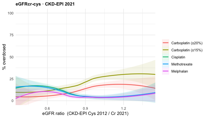
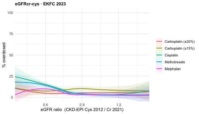
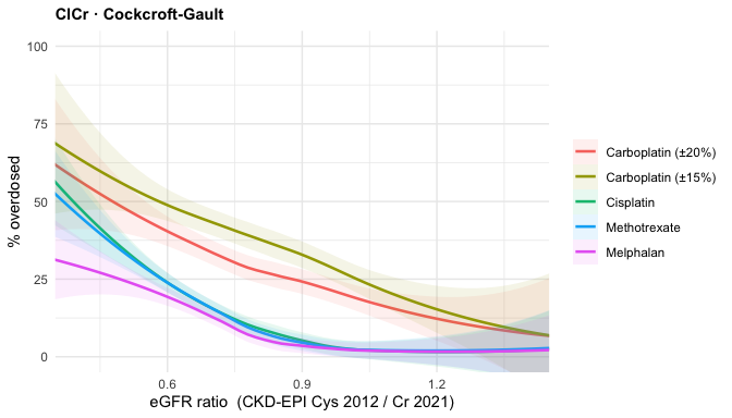
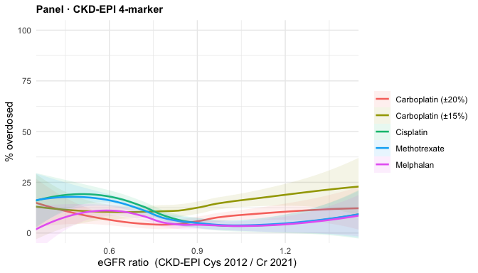
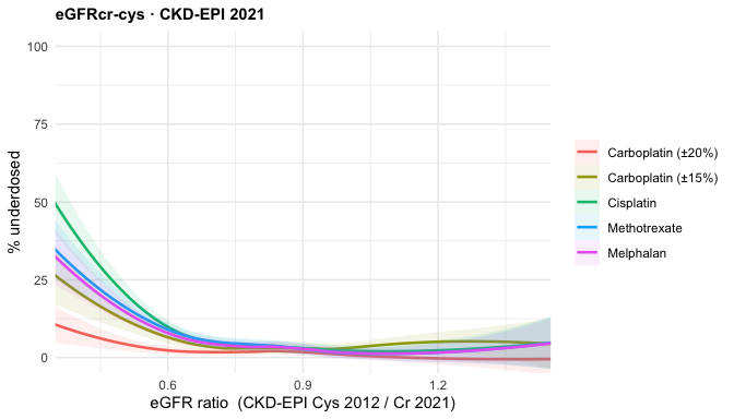
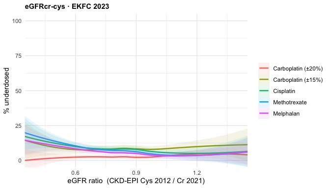
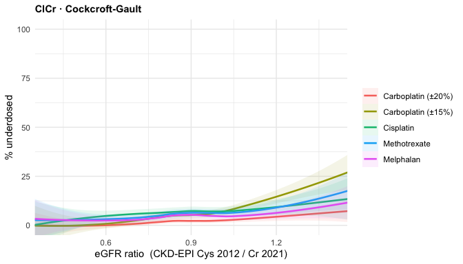
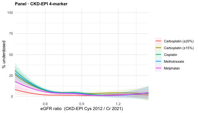
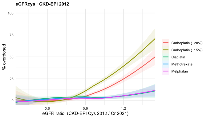
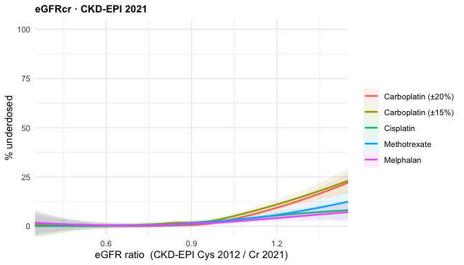
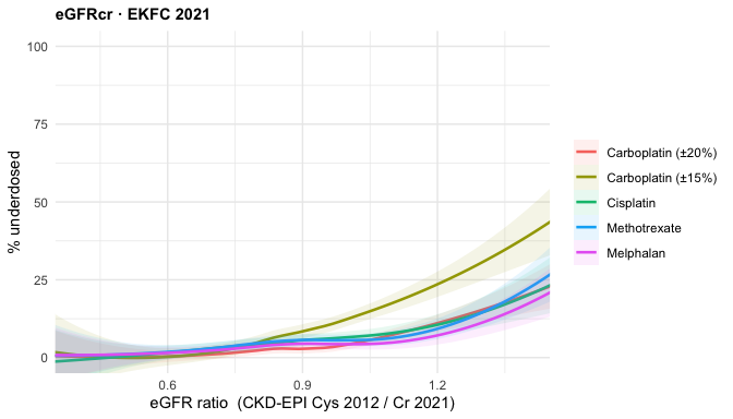
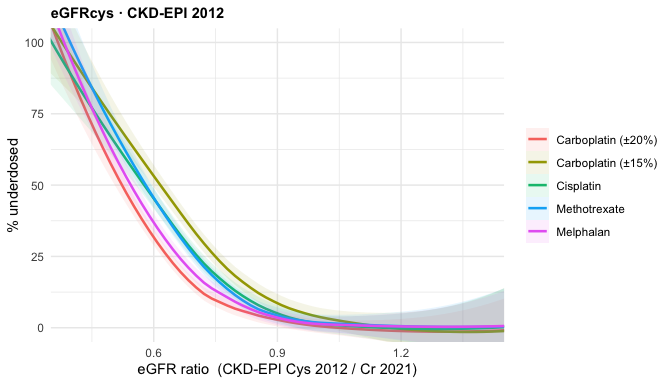
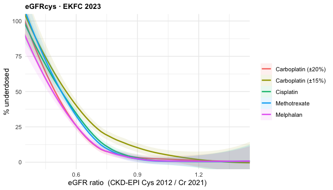
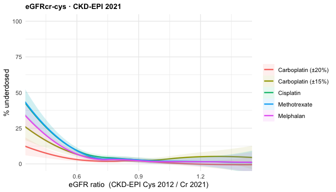
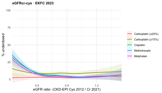
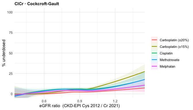
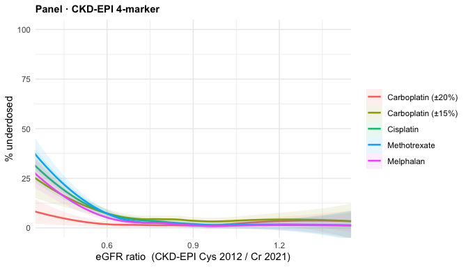
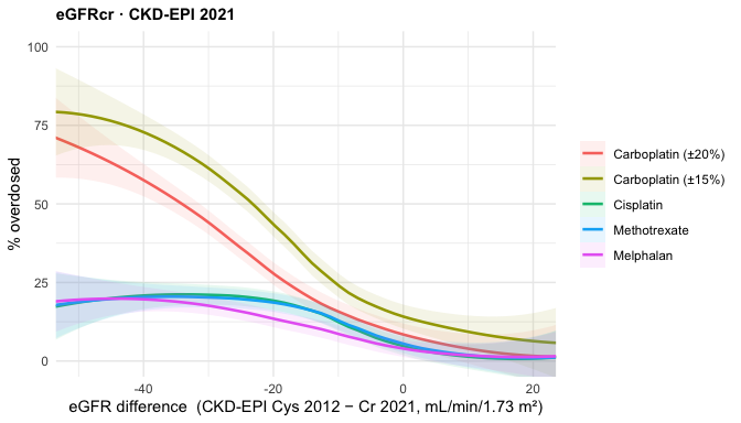
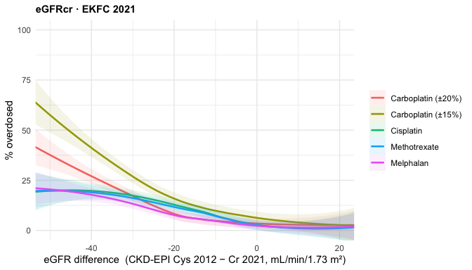
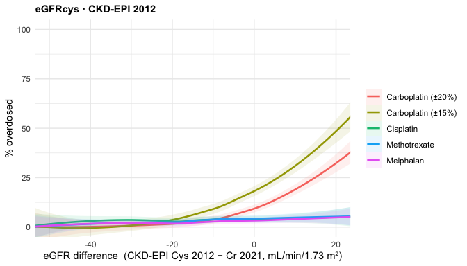
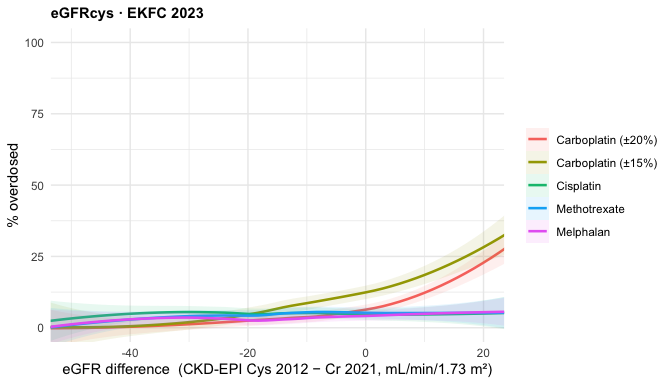
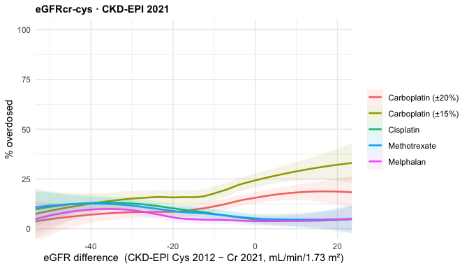
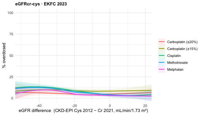
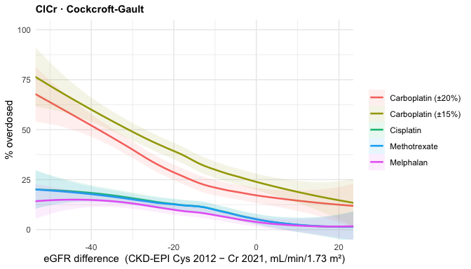
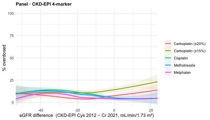
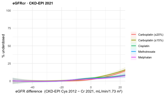
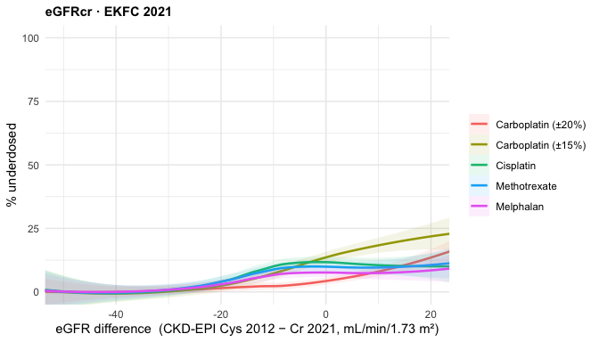
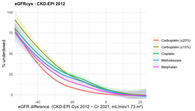
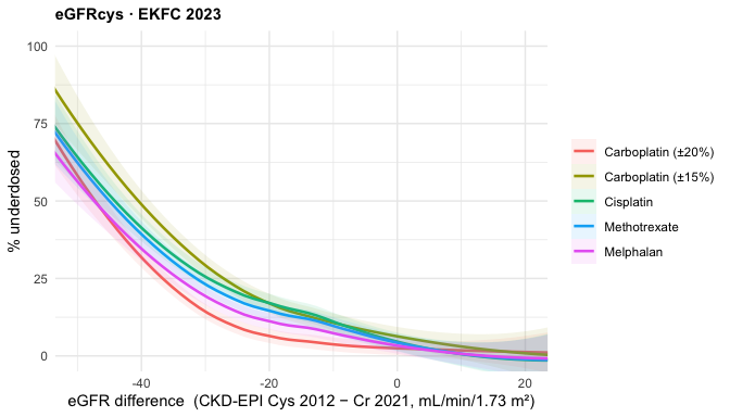
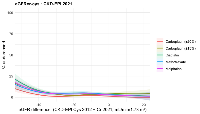
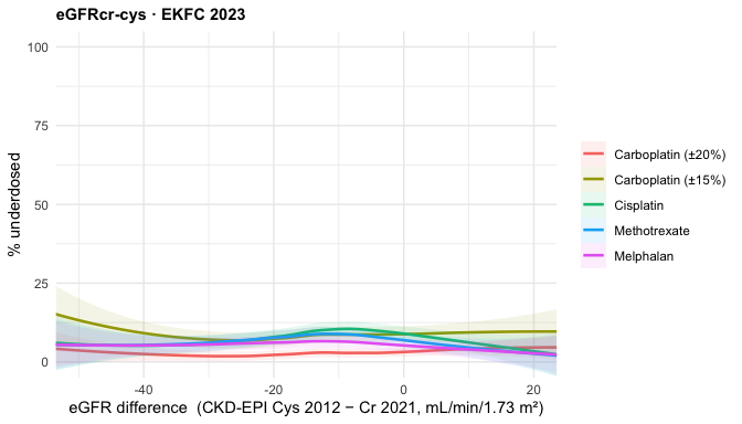
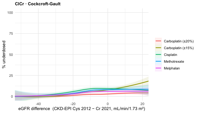
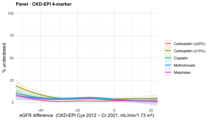
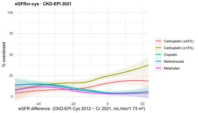
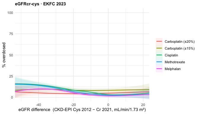
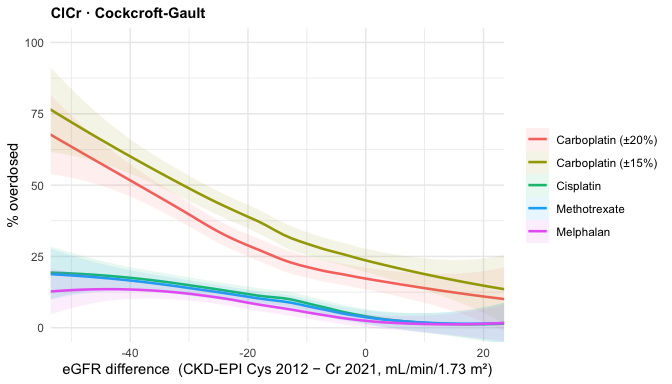
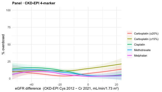
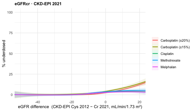
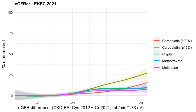
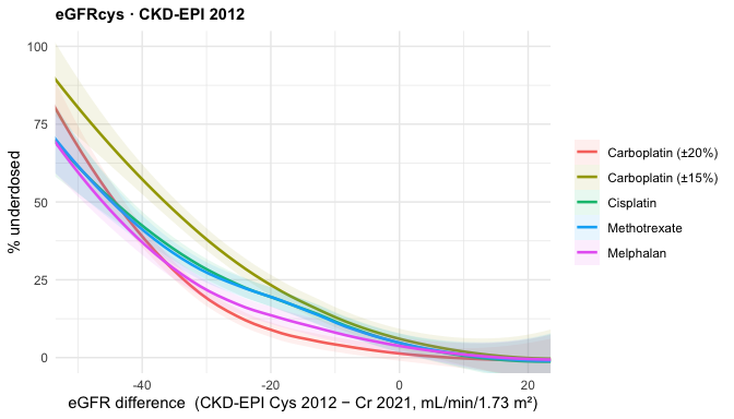
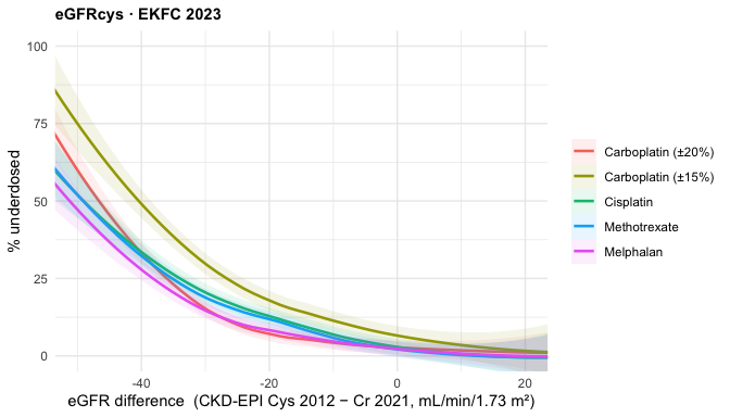
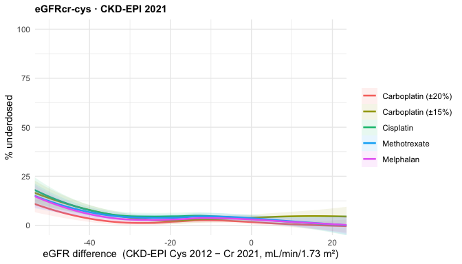
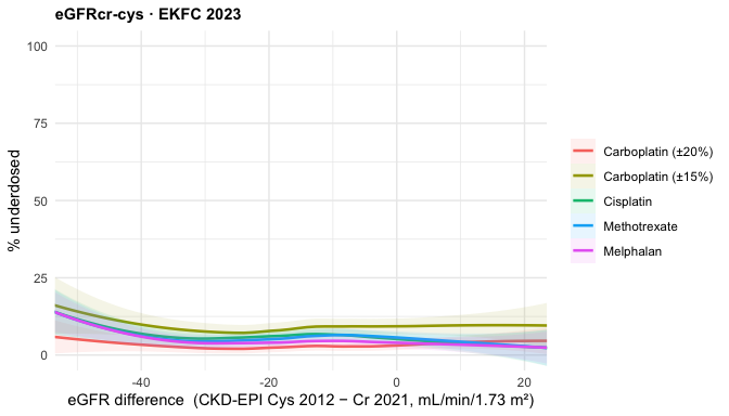
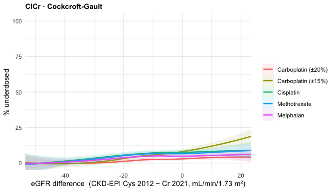
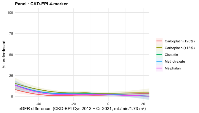
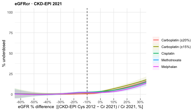
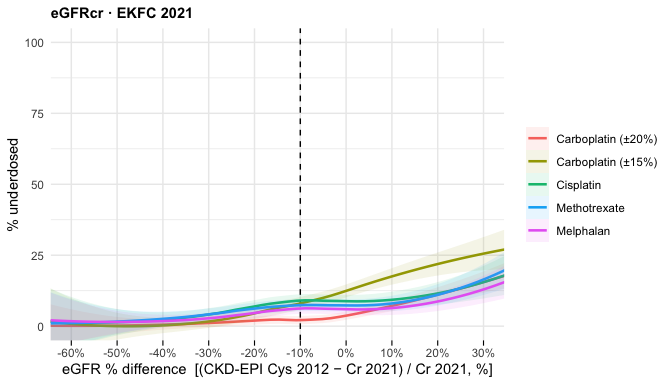
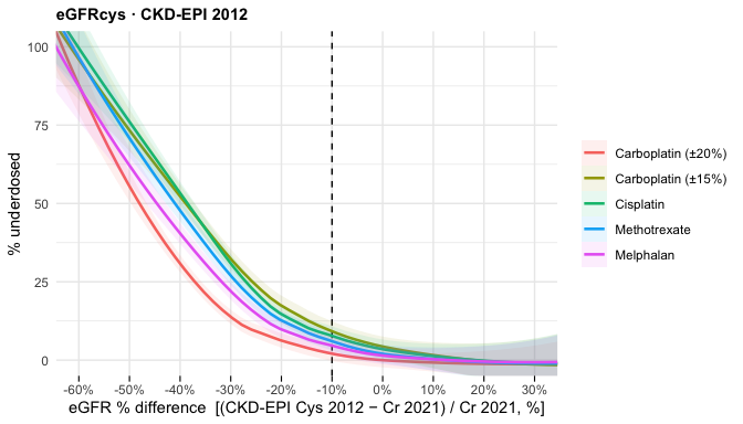
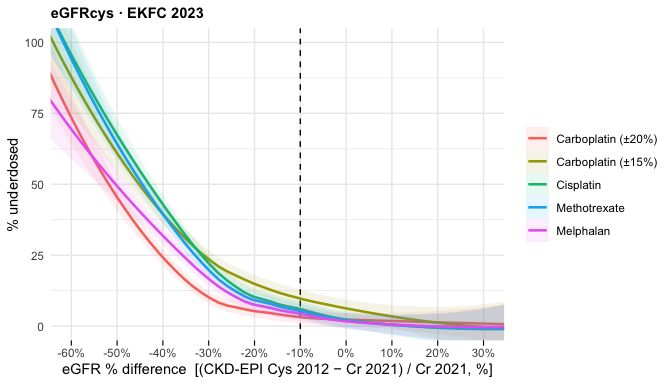
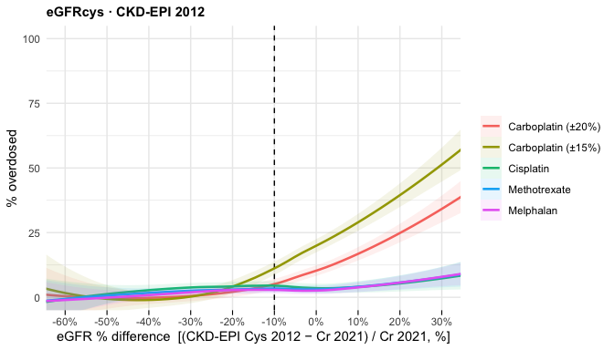
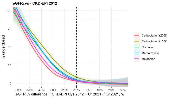
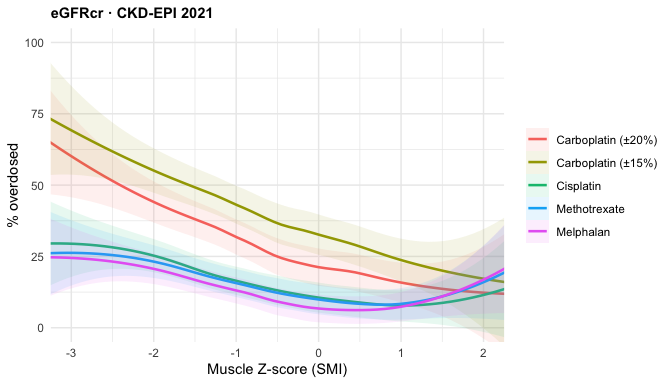
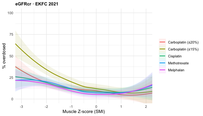
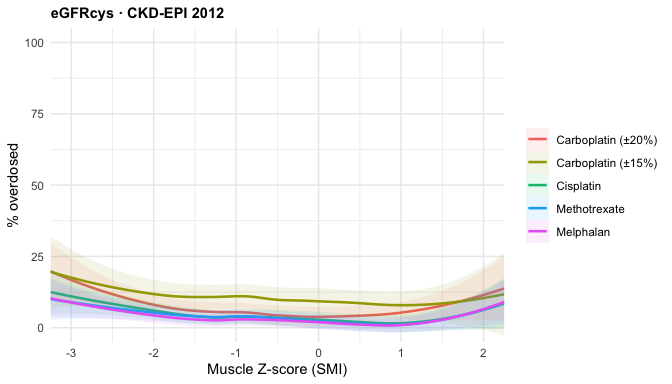
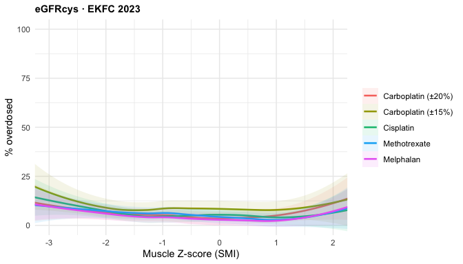
# Equations shown in the LOESS panels — all 8. NB: the CKD-EPI Cys 2012 and
# CKD-EPI Cr 2021 panels are partly self-referential (they define the x-axis
# ratio/difference), so interpret those two with care.
LOESS_EQS <- reg$equation

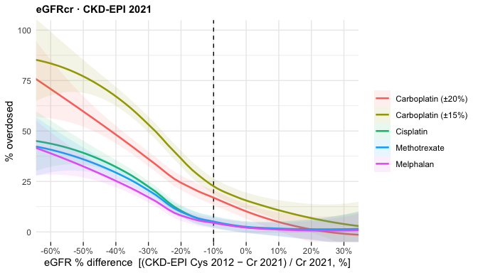
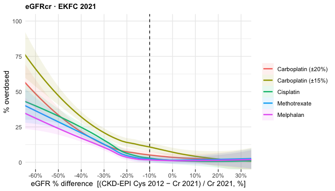
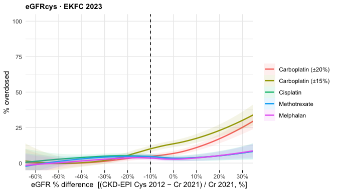
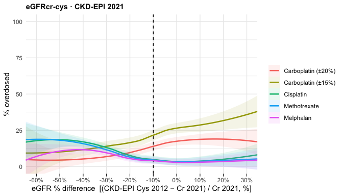
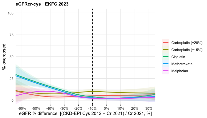
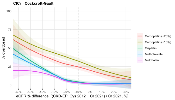
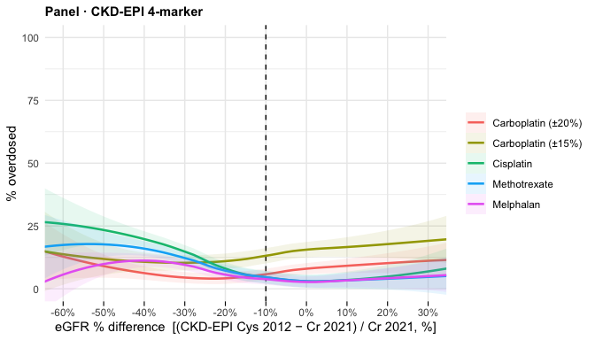
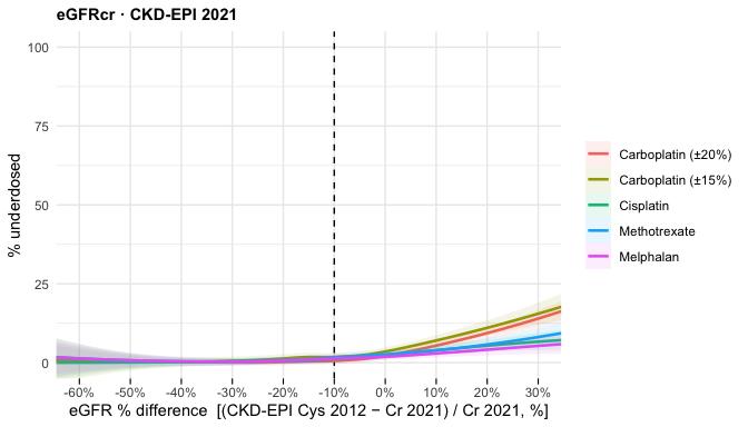
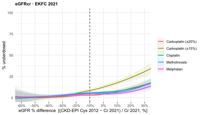
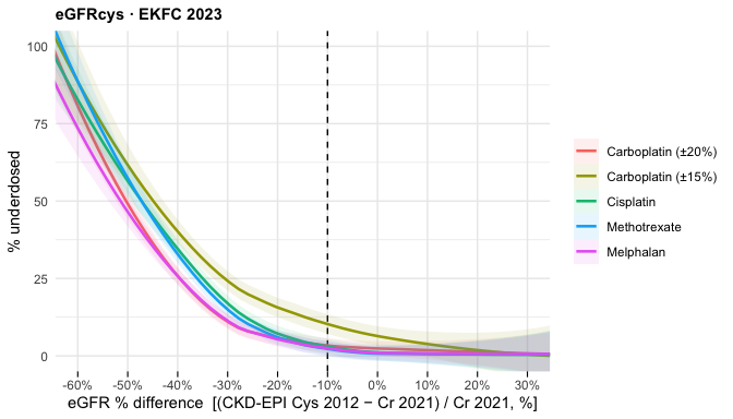
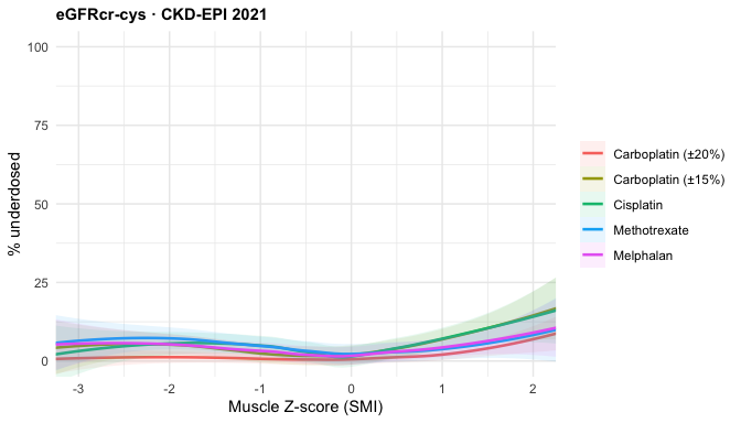
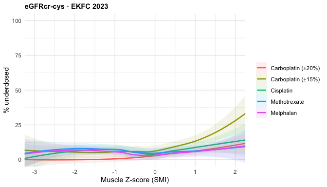
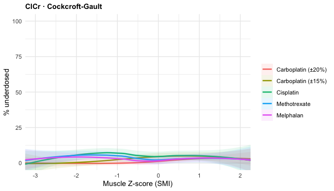
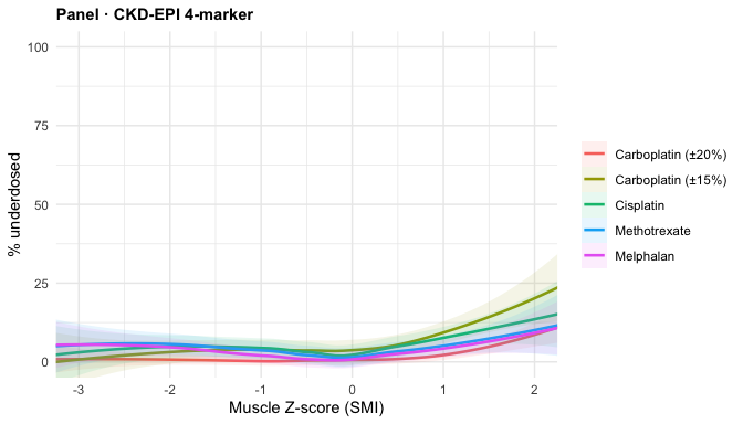
# LOESS: one plot per equation; the 5 drugs are overlaid as colour-coded LOESS
# smooths of P(over/under-dose) vs an x variable (binary 0/1 -> % via mean).
# `xvar`/`xlab`/`xlim` default to the eGFR ratio; the difference set overrides them.
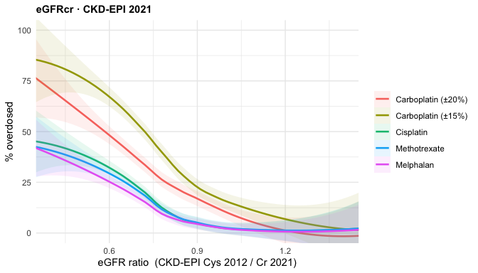
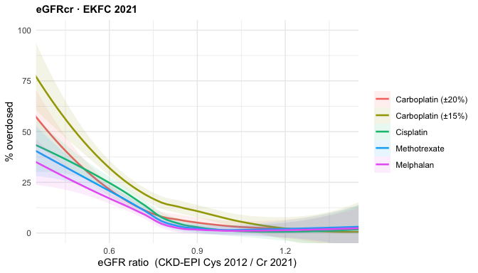
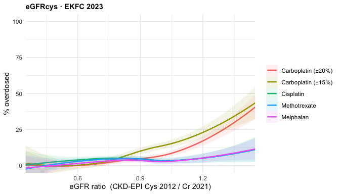
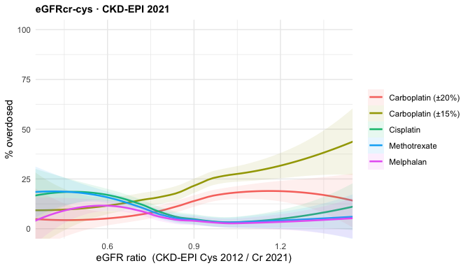
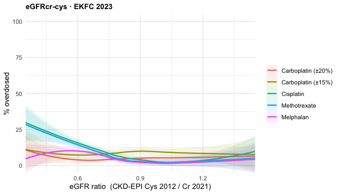
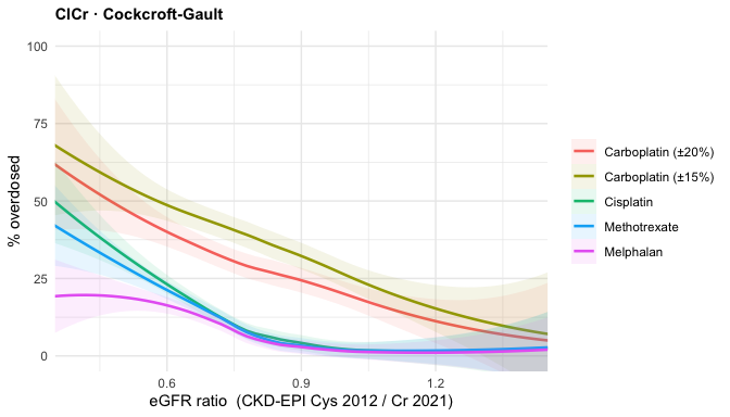
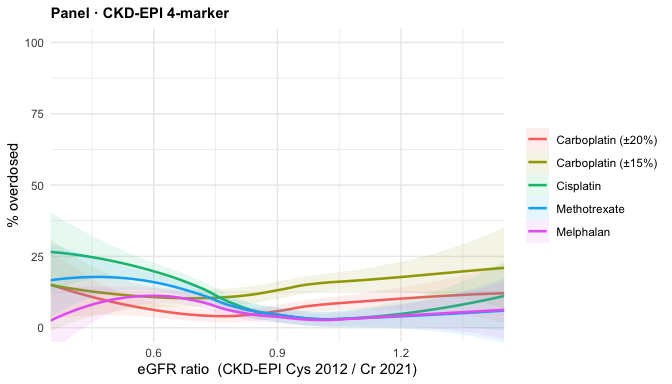
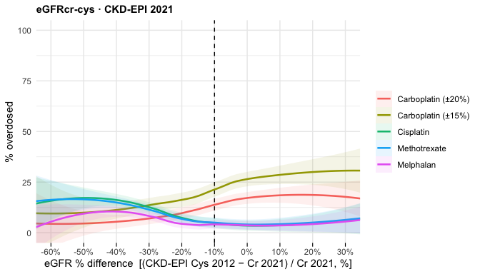
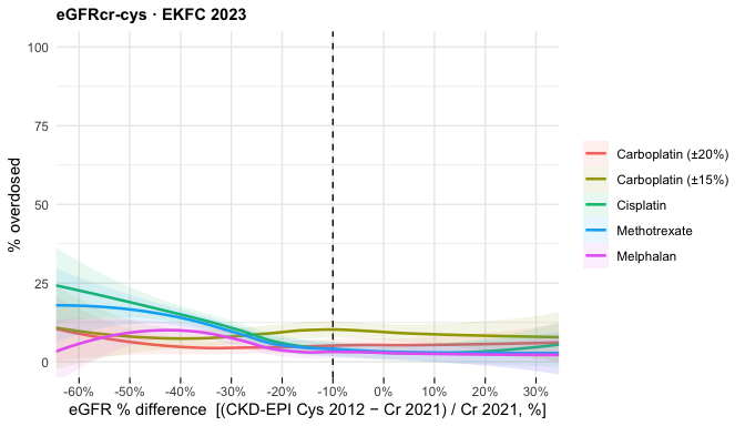
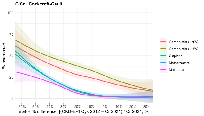
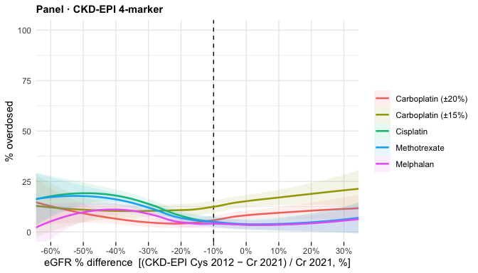
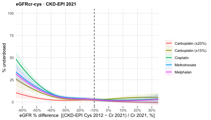
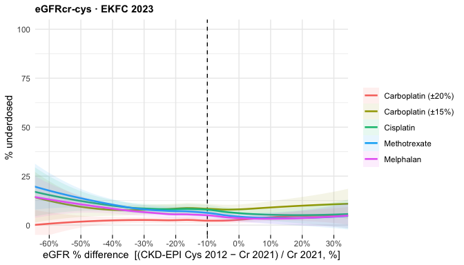
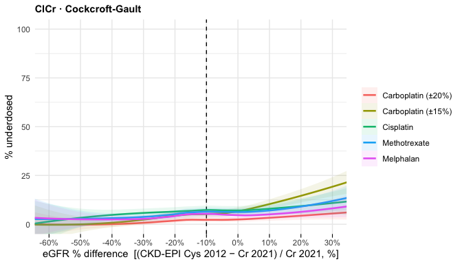
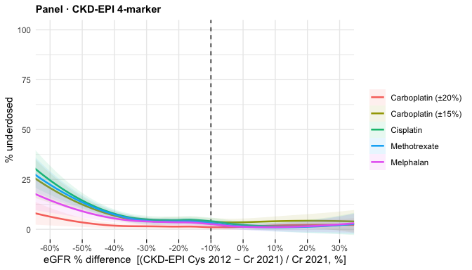
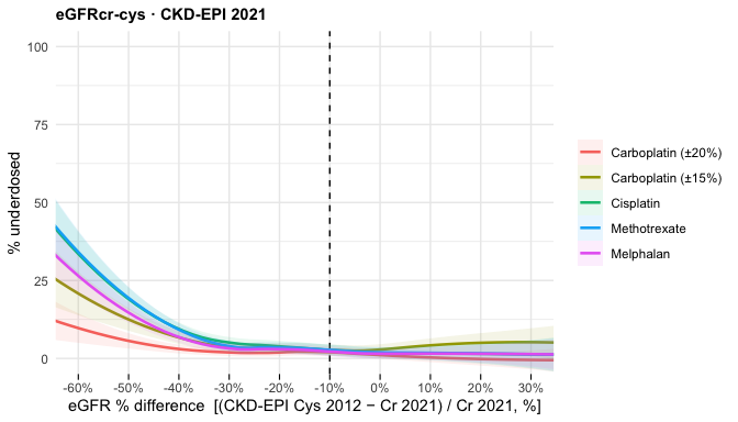
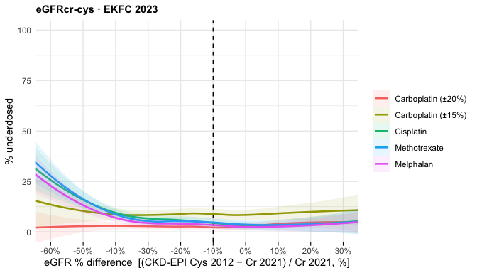
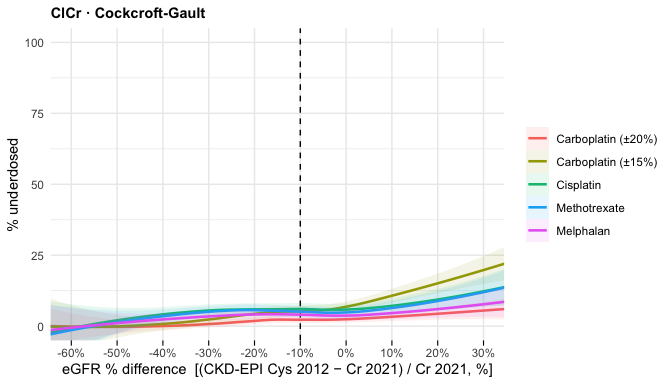
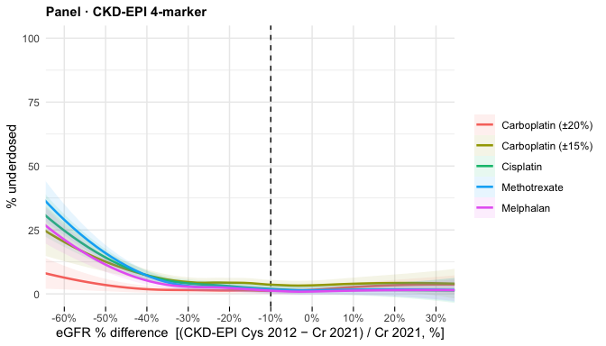
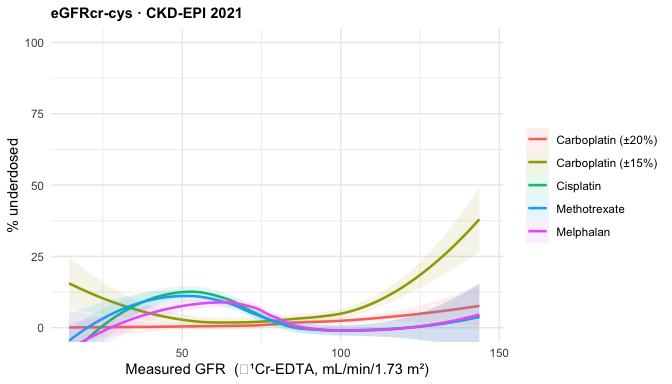
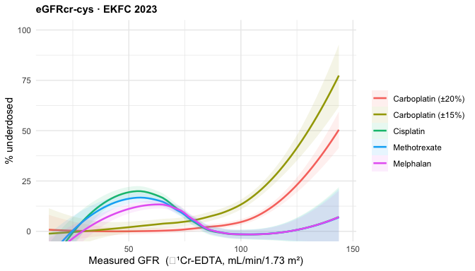
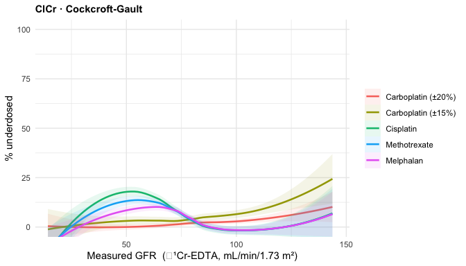
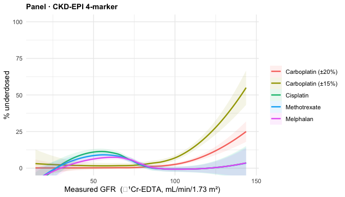
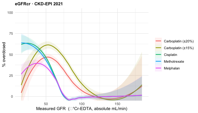
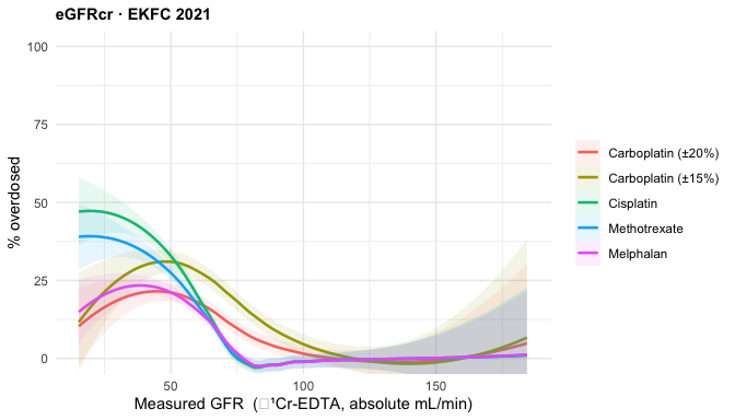
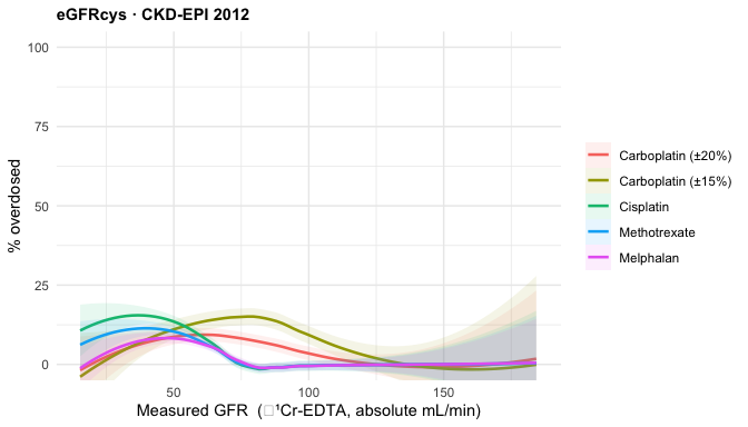
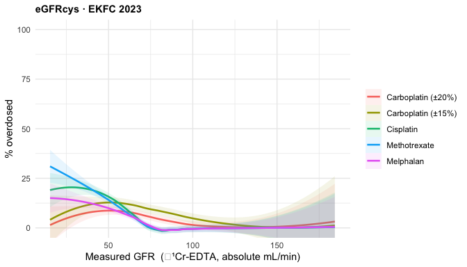
loess_plot <- function(cl, eq, direction, xvar = "egfr_ratio",
                       xlab = "eGFR ratio  (CKD-EPI Cys 2012 / Cr 2021)",
                       xlim = c(0.4, 1.4), pctd_axis = FALSE) {
  r   <- reg[reg$equation == eq, ]
  ttl <- paste0(r$type, " · ", r$label)
  d <- cl %>%
    dplyr::filter(equation == eq, !is.na(cls), !is.na(.data[[xvar]])) %>%
    dplyr::mutate(y = as.integer(cls == direction) * 100,
                  Drug = factor(drug, levels = DRUG_IDS, labels = DRUG_LABS))
  p <- ggplot2::ggplot(d, ggplot2::aes(.data[[xvar]], y, colour = Drug, fill = Drug))
  # pctd_axis = TRUE gives the Grant-page x axis: -10 % dashed marker under the
  # curves, 10-point ticks with % labels. Used by the % difference set only.
  if (pctd_axis) p <- p + ref_vline()
  p <- p +
    ggplot2::geom_smooth(method = "loess", formula = y ~ x, span = 0.9,
                         se = TRUE, alpha = 0.10, linewidth = 0.9) +
    ggplot2::coord_cartesian(xlim = xlim, ylim = c(0, 100)) +
    ggplot2::labs(x = xlab, y = paste0("% ", tolower(direction), "d"),
                  title = ttl, colour = NULL, fill = NULL) +
    ggplot2::theme_minimal(base_size = 11) +
    ggplot2::theme(legend.position = "right",
                   plot.title = ggplot2::element_text(face = "bold", size = 11))
  if (pctd_axis) p <- p + pctd_x()
  p
}
# X-axis for the difference LOESS set (indexed Cys − Cr, mL/min/1.73 m²).
DIFF_XLAB <- "eGFR difference  (CKD-EPI Cys 2012 − Cr 2021, mL/min/1.73 m²)"
DIFF_XLIM <- c(-50, 20)
# X-axis for the % difference LOESS set ((Cys − Cr)/Cr × 100; scale-invariant).
# Axis treatment copied from the Grant page — 10-point ticks with % labels and a
# black dashed marker at -10 % — but the window is sized to THIS index, which sits
# further negative than the Grant page's (median -16 %, range -69..+80):
# [-60, 30] holds 98.3 % of patients and keeps the smooth off the sparse tails.
PCTD_XLAB   <- "eGFR % difference  [(CKD-EPI Cys 2012 − Cr 2021) / Cr 2021, %]"
PCTD_XLIM   <- c(-60, 30)
PCTD_BREAKS <- seq(-80, 80, 10)   # spans the full data range; clipped panels drop the extras
REF_LINE    <- -10
BINW        <- 5                  # histogram bin width, percentage points
CARBO_RED   <- "#F8766D"          # ggplot's hue for the carboplatin ±20% line

pctd_x <- function() {
  list(
    ggplot2::scale_x_continuous(breaks = PCTD_BREAKS,
                                labels = paste0(PCTD_BREAKS, "%"),
                                minor_breaks = NULL),
    ggplot2::theme(
      axis.ticks.x        = ggplot2::element_line(colour = "black", linewidth = 0.4),
      axis.ticks.length.x = grid::unit(4, "pt"),
      panel.grid.minor.x  = ggplot2::element_blank()))
}
ref_vline <- function() {
  ggplot2::geom_vline(xintercept = REF_LINE, linetype = "dashed",
                      colour = "black", linewidth = 0.5)
}

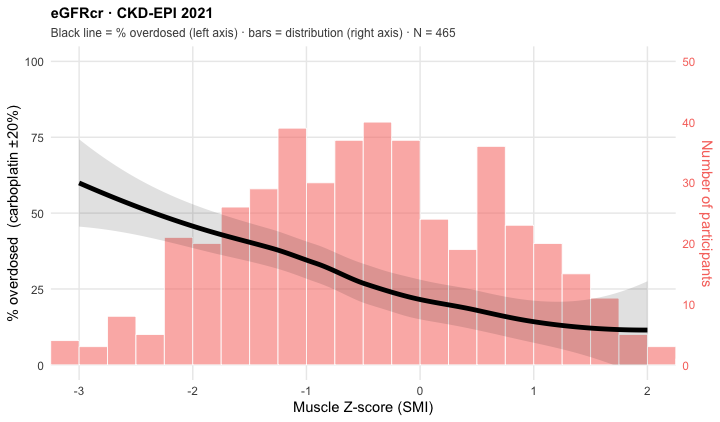
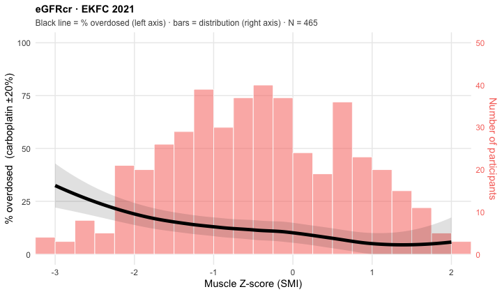
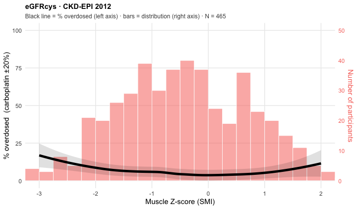
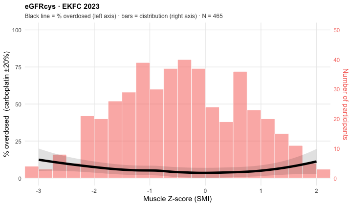
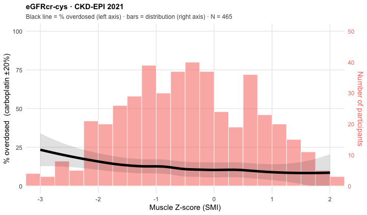
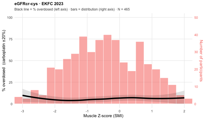
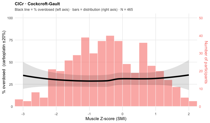
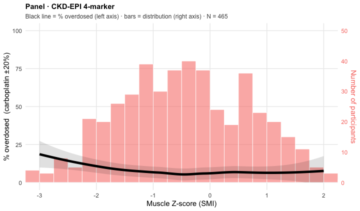
# Overdose curve superimposed on the cohort distribution — the Grant page's
# Figure 3, generalised to any equation. Carboplatin ±20 % overdose LOESS (black,
# thick, left axis 0-100 %) over a histogram of the x variable (bars, right axis
# = count). Bars are drawn as a fraction of the tallest bin (rounded up to a clean
# 25) so both series share one panel; the right axis inverts that transform.
# The curve is clipped to [0, 100] exactly as on the Grant page.
overlay_plot <- function(cl, eq, xvar = "egfr_pctdiff", xlab = PCTD_XLAB,
                         xlim = PCTD_XLIM, drug_id = "carboplatin_b20",
                         binw = BINW, pct_axis = TRUE, ref_at = REF_LINE,
                         data = dat) {
  r   <- reg[reg$equation == eq, ]
  ttl <- paste0(r$type, " · ", r$label)

  xall  <- data[[xvar]]; xall <- xall[!is.na(xall)]
  n_tot <- length(xall)
  brks  <- seq(floor(min(xall) / binw) * binw, ceiling(max(xall) / binw) * binw, binw)
  cnt_max <- .nice_max(max(graphics::hist(xall, breaks = brks, plot = FALSE)$counts))

  d <- cl %>%
    dplyr::filter(equation == eq, drug == drug_id, !is.na(cls), !is.na(.data[[xvar]])) %>%
    dplyr::mutate(y = as.integer(cls == "Overdose") * 100)
  fit  <- stats::loess(y ~ x, span = 0.9, data = data.frame(x = d[[xvar]], y = d$y))
  gx   <- seq(xlim[1], xlim[2], length.out = 200)
  pr   <- stats::predict(fit, newdata = data.frame(x = gx), se = TRUE)
  clip <- function(v) pmin(pmax(v, 0), 100)
  ov   <- data.frame(x = gx, fit = clip(pr$fit),
                     lo = clip(pr$fit - 1.96 * pr$se.fit),
                     hi = clip(pr$fit + 1.96 * pr$se.fit))

  p <- ggplot2::ggplot() +
    ggplot2::geom_histogram(
      data = data.frame(x = xall),
      ggplot2::aes(x, y = ggplot2::after_stat(count) / cnt_max * 100),
      binwidth = binw, boundary = 0,
      fill = CARBO_RED, colour = "white", linewidth = 0.3, alpha = 0.55)
  if (!is.null(ref_at))
    p <- p + ggplot2::geom_vline(xintercept = ref_at, linetype = "dashed",
                                 colour = "black", linewidth = 0.5)
  p <- p +
    ggplot2::geom_ribbon(data = ov, ggplot2::aes(x, ymin = lo, ymax = hi),
                         fill = "black", alpha = 0.12) +
    ggplot2::geom_line(data = ov, ggplot2::aes(x, y = fit),
                       colour = "black", linewidth = 1.7)
  if (pct_axis) p <- p + pctd_x()
  p +
    ggplot2::scale_y_continuous(
      name = "% overdosed  (carboplatin ±20%)", breaks = seq(0, 100, 25),
      sec.axis = ggplot2::sec_axis(~ . / 100 * cnt_max, name = "Number of participants",
                                   breaks = scales::pretty_breaks(5))) +
    ggplot2::coord_cartesian(xlim = xlim, ylim = c(0, 100)) +
    ggplot2::labs(
      x = xlab, title = ttl,
      subtitle = sprintf("Black line = %% overdosed (left axis) · bars = distribution (right axis) · N = %s",
                         format(n_tot, big.mark = ","))) +
    .overlay_theme()
}

# Shared look for every panel in the "Carboplatin 20 % plots" section: pink
# distribution on the right axis, black overdose series on the left.
.overlay_theme <- function() {
  ggplot2::theme_minimal(base_size = 11) +
    ggplot2::theme(
      plot.title         = ggplot2::element_text(face = "bold", size = 11),
      plot.subtitle      = ggplot2::element_text(size = 9, colour = "grey30"),
      axis.title.y.right = ggplot2::element_text(colour = CARBO_RED),
      axis.text.y.right  = ggplot2::element_text(colour = CARBO_RED),
      panel.grid.minor   = ggplot2::element_blank())
}
# Round a count up to a clean axis maximum, with ~15 % headroom so the tallest
# bar stops short of the panel top and the black overdose line stays readable
# over it. Step scales with magnitude.
.nice_max <- function(mx) {
  mx   <- mx * 1.15
  step <- if (mx <= 20) 5 else if (mx <= 50) 10 else 25
  ceiling(mx / step) * step
}

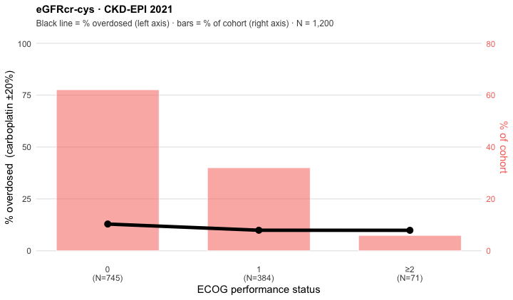
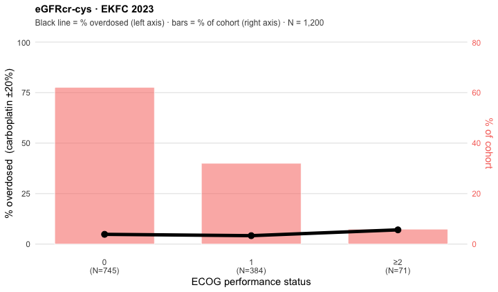
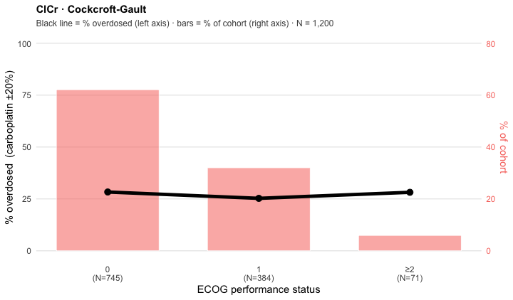
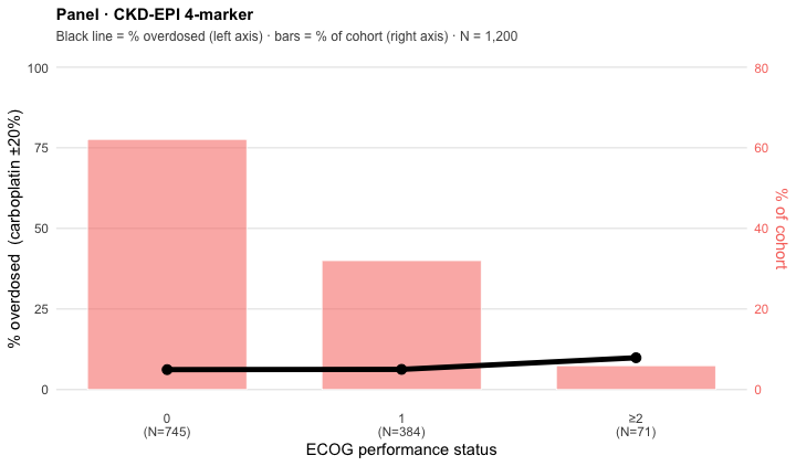
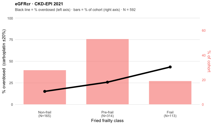
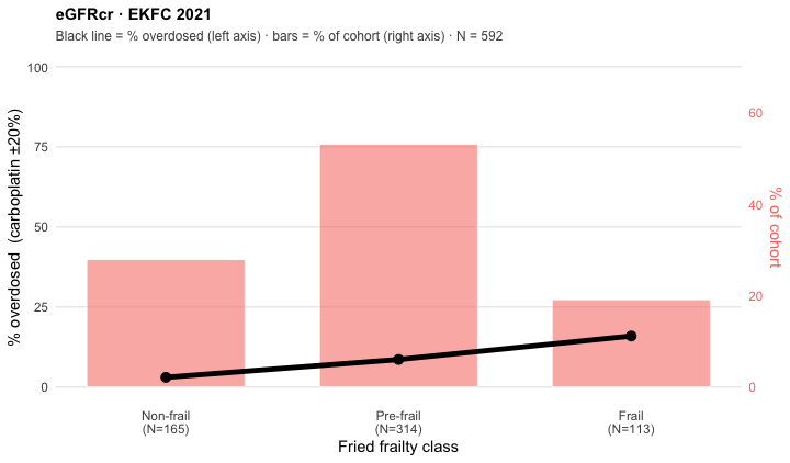
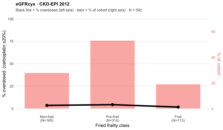
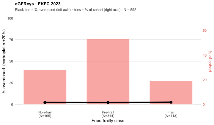
# Discrete-marker twin of overlay_plot: bars = the share of the cohort in each
# category (pink, right axis); black line+points = the share of that category
# overdosed (left axis). Same colours, axes and theme as the continuous panels,
# so the four markers read as one set.
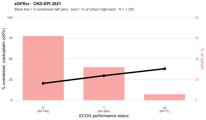
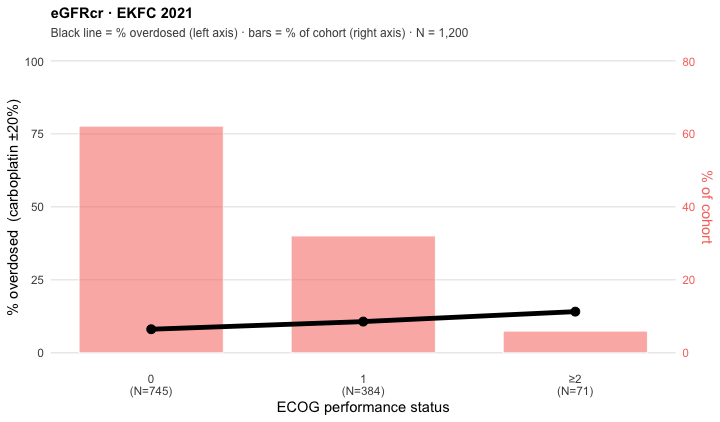
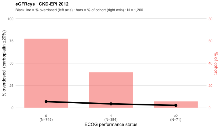
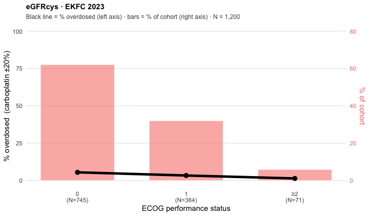
bar_line_plot <- function(cl, eq, grpcol, xlab, drug_id = "carboplatin_b20") {
  r   <- reg[reg$equation == eq, ]
  ttl <- paste0(r$type, " · ", r$label)
  agg <- cl %>%
    dplyr::filter(equation == eq, drug == drug_id, !is.na(cls), !is.na(.data[[grpcol]])) %>%
    dplyr::mutate(grp = droplevels(.data[[grpcol]])) %>%
    dplyr::group_by(grp) %>%
    dplyr::summarise(N = dplyr::n(),
                     pct_over = mean(cls == "Overdose") * 100, .groups = "drop") %>%
    dplyr::arrange(grp) %>%
    dplyr::mutate(pct_cohort = N / sum(N) * 100)
  n_tot   <- sum(agg$N)
  cnt_max <- ceiling(max(agg$pct_cohort) * 1.15 / 10) * 10   # headroom, as above
  xl <- paste0(levels(agg$grp), "\n(N=", agg$N, ")")

  ggplot2::ggplot(agg, ggplot2::aes(x = as.integer(grp))) +
    ggplot2::geom_col(ggplot2::aes(y = pct_cohort / cnt_max * 100),
                      fill = CARBO_RED, colour = "white", linewidth = 0.3,
                      alpha = 0.55, width = 0.68) +
    ggplot2::geom_line(ggplot2::aes(y = pct_over), colour = "black", linewidth = 1.7) +
    ggplot2::geom_point(ggplot2::aes(y = pct_over), colour = "black", size = 2.8) +
    ggplot2::scale_x_continuous(breaks = seq_along(xl), labels = xl) +
    ggplot2::scale_y_continuous(
      name = "% overdosed  (carboplatin ±20%)", breaks = seq(0, 100, 25),
      sec.axis = ggplot2::sec_axis(~ . / 100 * cnt_max, name = "% of cohort",
                                   breaks = scales::pretty_breaks(5))) +
    ggplot2::coord_cartesian(ylim = c(0, 100)) +
    ggplot2::labs(
      x = xlab, title = ttl,
      subtitle = sprintf("Black line = %% overdosed (left axis) · bars = %% of cohort (right axis) · N = %s",
                         format(n_tot, big.mark = ","))) +
    .overlay_theme() +
    ggplot2::theme(panel.grid.major.x = ggplot2::element_blank())
}
# X-axis for the measured-GFR LOESS set (the reference itself; indexed vs absolute).
MGFR_XLAB_IDX <- "Measured GFR  (⁵¹Cr-EDTA, mL/min/1.73 m²)"
MGFR_XLIM_IDX <- c(15, 145)
MGFR_XLAB_NIX <- "Measured GFR  (⁵¹Cr-EDTA, absolute mL/min)"
MGFR_XLIM_NIX <- c(15, 185)
# X-axis for the muscle Z-score LOESS (465 body-comp cohort).
MZ_XLAB <- "Muscle Z-score (SMI)"
MZ_XLIM <- c(-3, 2)

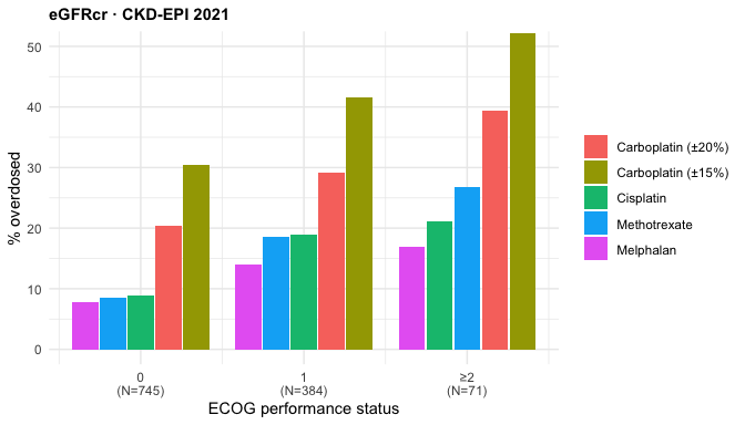
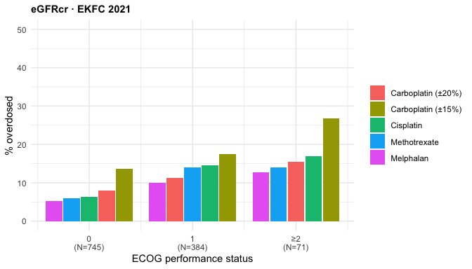
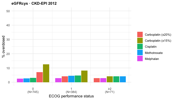
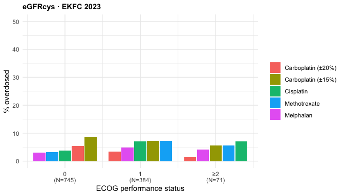
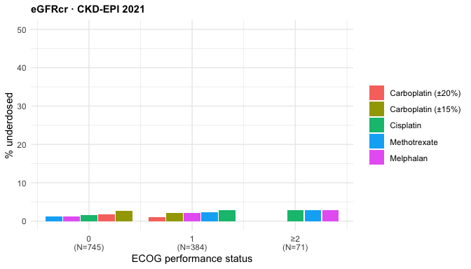
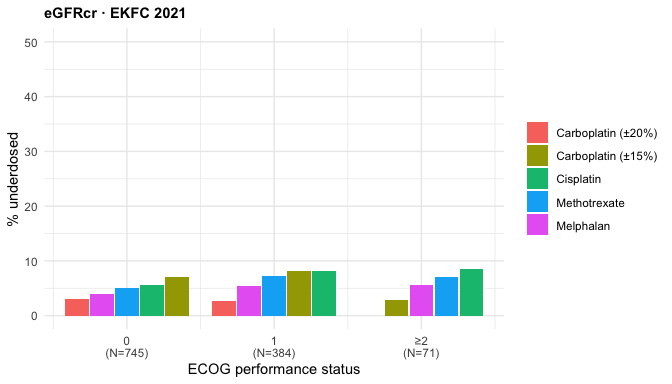
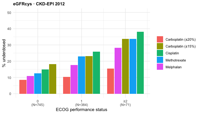
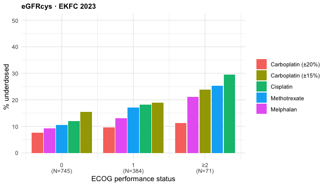
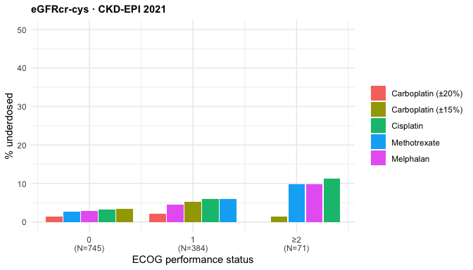
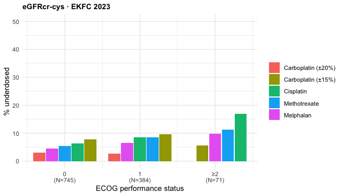
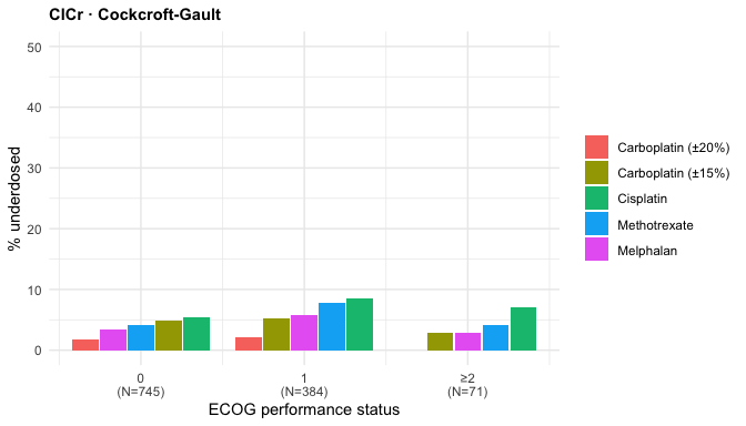
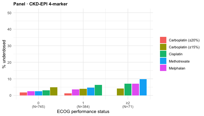
# ECOG distribution: % over/under-dose by ECOG group (0 / 1 / ≥2), one line per
# drug, per equation. N per ECOG group is annotated on the x-axis labels.
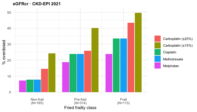
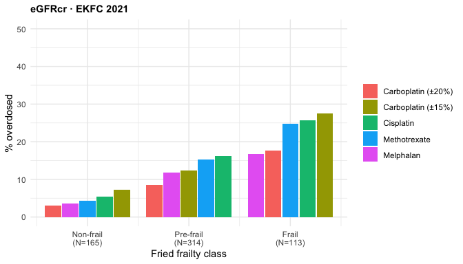
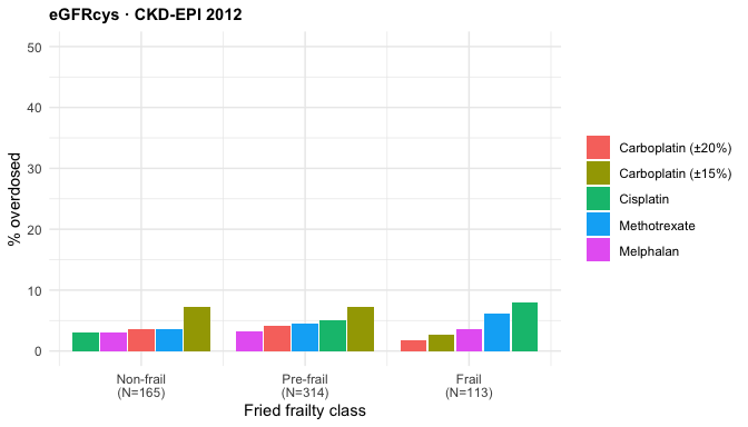
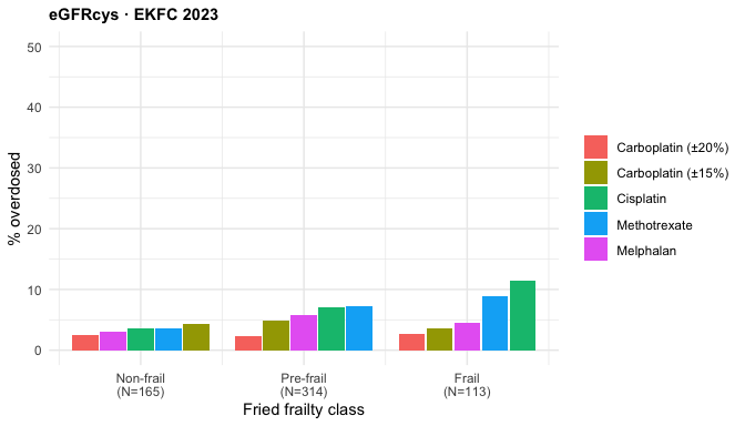
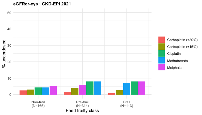
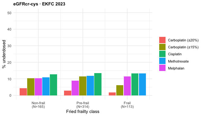
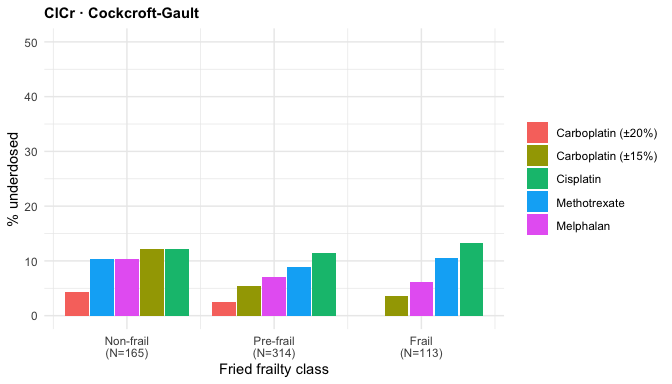
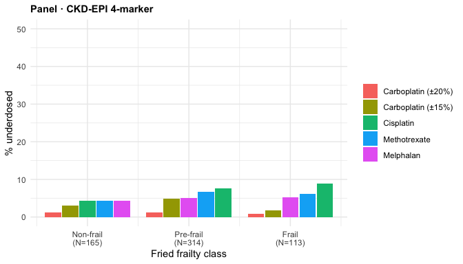
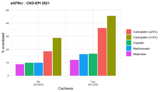
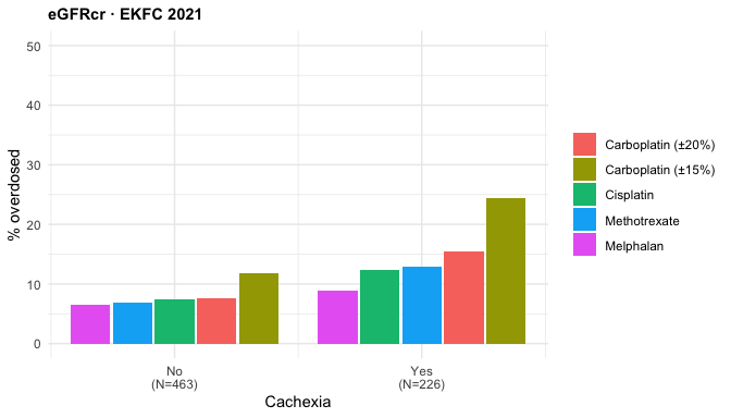
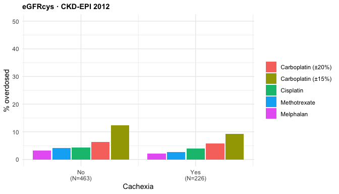
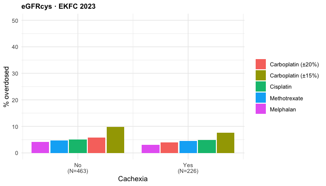
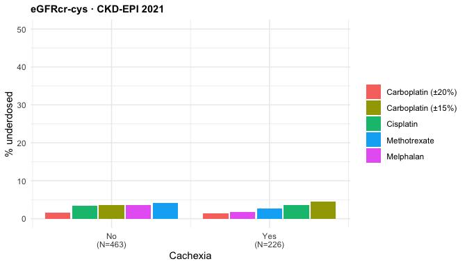
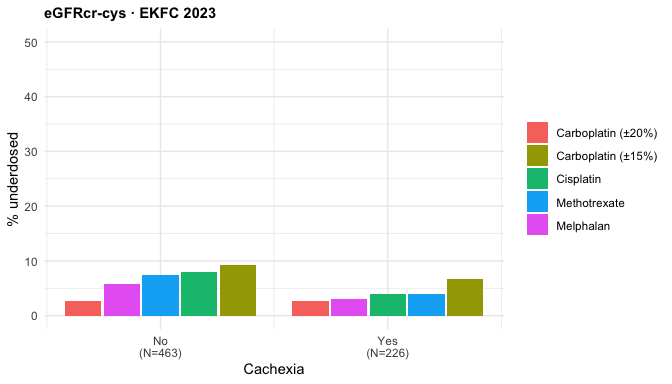
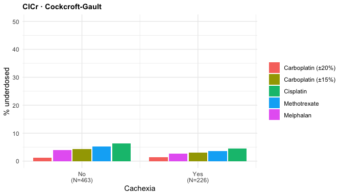
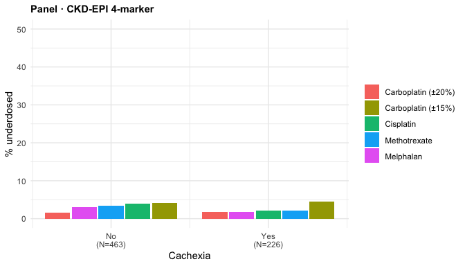
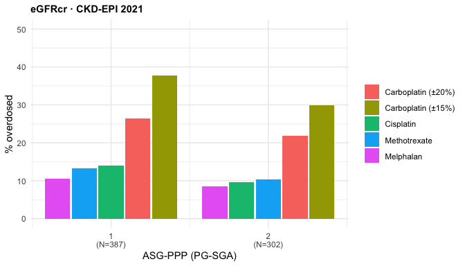
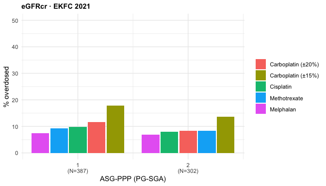
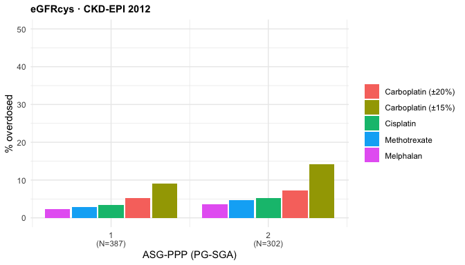
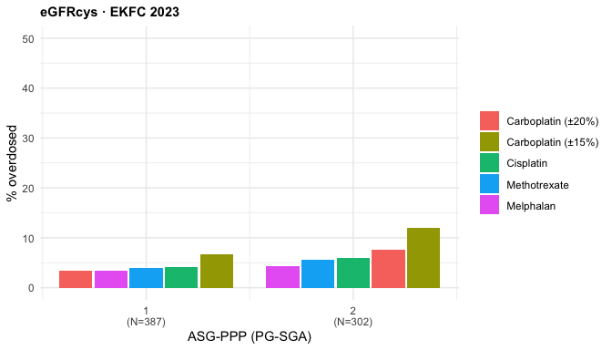
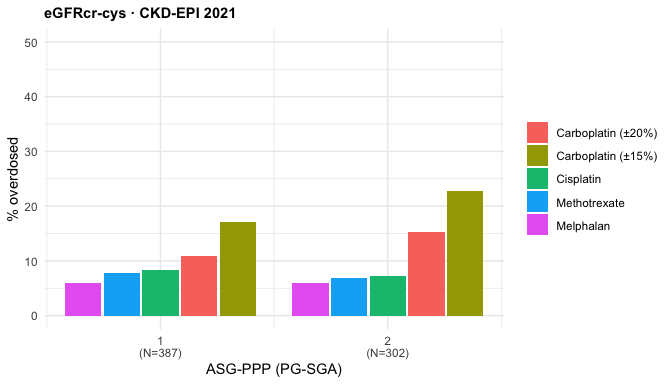
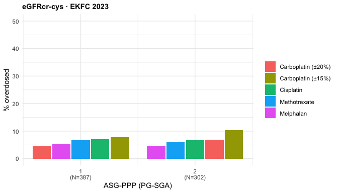
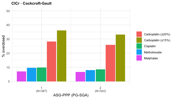
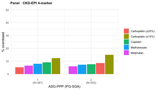
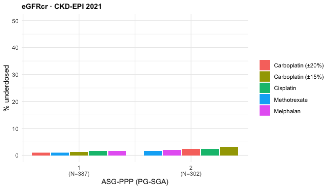
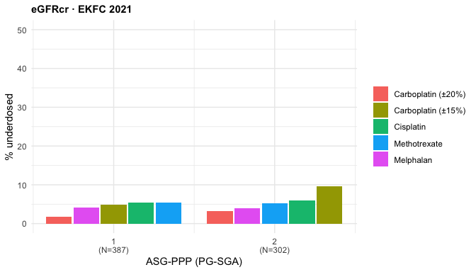
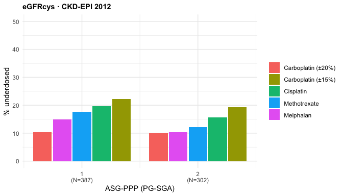
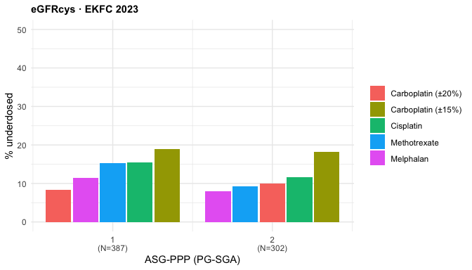
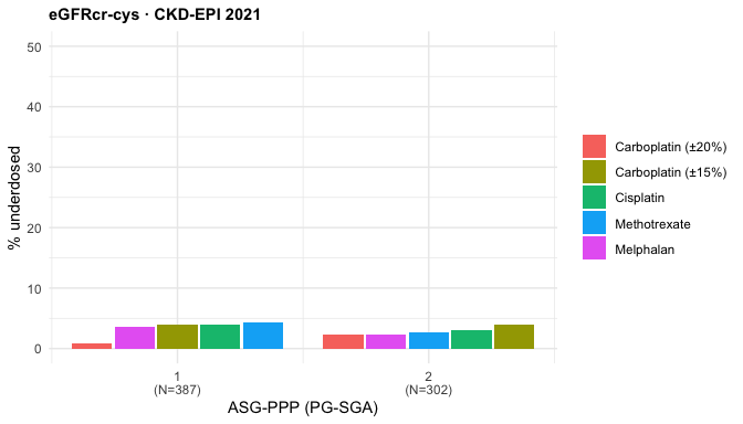
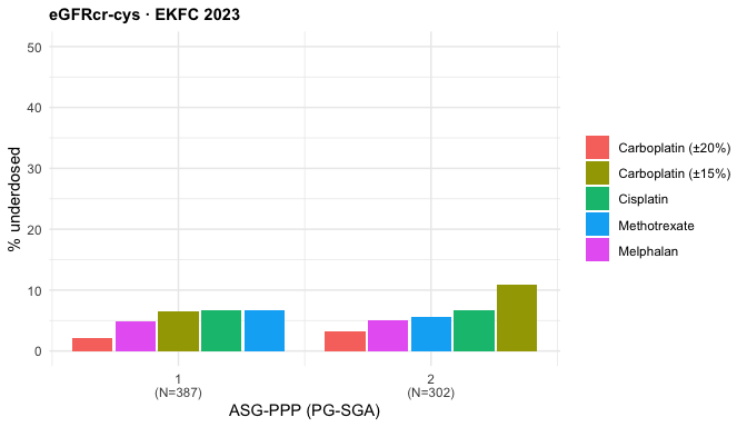
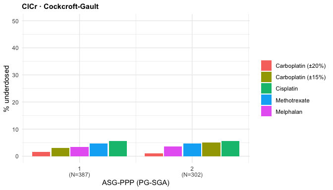
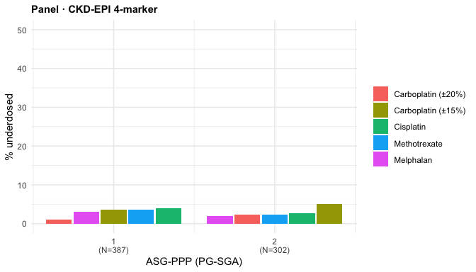
# Grouped-bar plot of % over/under-dose by a categorical group (`grpcol`); 5 drug
# bars per group, sorted low->high. Used for ECOG and Fried frailty.
ecog_plot <- function(cl, eq, direction, grpcol = "ecog_grp", xlab = "ECOG performance status", ymax = NA) {
  r <- reg[reg$equation == eq, ]; ttl <- paste0(r$type, " · ", r$label)
  s <- cl %>%
    dplyr::filter(equation == eq, !is.na(cls), !is.na(.data[[grpcol]])) %>%
    dplyr::mutate(Drug = factor(drug, levels = DRUG_IDS, labels = DRUG_LABS),
                  grp  = .data[[grpcol]])
  agg <- s %>% dplyr::group_by(grp, Drug) %>%
    dplyr::summarise(pct = mean(cls == direction) * 100, .groups = "drop_last") %>%
    dplyr::arrange(pct, .by_group = TRUE) %>%        # low -> high within each group
    dplyr::mutate(xpos = as.integer(grp) + (dplyr::row_number() - 3) * 0.17) %>%
    dplyr::ungroup()
  ns <- s %>% dplyr::filter(drug == DRUG_IDS[1]) %>% dplyr::count(grp)
  xl <- paste0(levels(s$grp), "\n(N=",
               ns$n[match(levels(s$grp), as.character(ns$grp))], ")")
  ggplot2::ggplot(agg, ggplot2::aes(xpos, pct, fill = Drug)) +
    ggplot2::geom_col(width = 0.16) +
    ggplot2::scale_x_continuous(breaks = seq_along(xl), labels = xl) +
    ggplot2::coord_cartesian(ylim = c(0, ymax)) +
    ggplot2::labs(x = xlab, y = paste0("% ", tolower(direction), "d"),
                  title = ttl, fill = NULL) +
    ggplot2::theme_minimal(base_size = 11) +
    ggplot2::theme(legend.position = "right",
                   plot.title = ggplot2::element_text(face = "bold", size = 11))
}

# Emit every drug × direction for one scale/version (call inside a results='asis'
# chunk). Saves each table to Word and prints it with a download link.
emit_scale <- function(cl, version, scale, scale_label, extra = FALSE, prefix = version) {
  cat("\n\n### ", scale_label, "\n\n", sep = "")
  for (d in DRUGS) {
    cat("\n\n#### ", d$lab, "\n\n", sep = "")
    for (dir in c("Overdose", "Underdose")) {
      fname <- paste0(prefix, "_", scale, "_", d$id, "_", tolower(dir))
      ft <- build_ft(cl, d$id, dir, version, extra)
      save_ft_docx(ft, fname)
      cat(flextable::flextable_to_rmd(ft))
      cat("\n\n")
    }
    cat(sprintf(
      "[📄 Overdose Word](../tables/heatmap/%1$s_%2$s_%3$s_overdose.docx) · [📄 Underdose Word](../tables/heatmap/%1$s_%2$s_%3$s_underdose.docx)\n\n",
      prefix, scale, d$id))
  }
}

# --- Most conservative GFR = per-patient MINIMUM of CKD-EPI Cr 2021,
# Cockcroft-Gault, and CKD-EPI Cr-Cys 2021 (the lowest / dose-limiting estimate).
build_mcg_long <- function(scale) {
  col_of <- function(eq) {
    r <- reg[reg$equation == eq, ]
    if (scale == "index") r$index_col[[1]] else r$nonindex_col[[1]]
  }
  mgfr <- dat[[MGFR[[scale]]]]
  mcg  <- pmin(dat[[col_of("CKDEPIcr21")]], dat[[col_of("CG")]],
               dat[[col_of("CKDEPIcrcys21")]], na.rm = TRUE)
  base <- dplyr::select(dat, sex, bmi_grp, met_grp, age_grp)
  tier <- purrr::map_dfr(TIER_DRUGS, function(dr)
    dplyr::bind_cols(base, tibble::tibble(drug = dr, cls = dose_class_tier(mcg, mgfr, dr))))
  carbo <- purrr::map_dfr(names(CARBO_BANDS), function(bn) {
    k <- CARBO_BANDS[[bn]]
    dplyr::bind_cols(base, tibble::tibble(drug = bn,
                                          cls = carbo_class(mcg, mgfr, k[["k_hi"]], k[["k_lo"]])))
  })
  dplyr::bind_rows(tier, carbo)
}
mcg_index    <- build_mcg_long("index")
mcg_nonindex <- build_mcg_long("nonindex")

# One table: rows = drugs, columns = subgroups, for the most-conservative GFR.
mcg_table <- function(cl, direction) {
  pct <- function(x) if (nrow(x)) round(mean(x$cls == direction) * 100, 1) else NA_real_
  lvl <- function(x, col, v) pct(x[!is.na(x[[col]]) & x[[col]] == v, ])
  per_drug <- function(dr) {
    e <- cl[cl$drug == dr, ]
    tibble::tibble(drug = dr, Overall = pct(e),
      Female = lvl(e, "sex", "Female"), Male = lvl(e, "sex", "Male"),
      bmi1 = lvl(e, "bmi_grp", "<20"), bmi2 = lvl(e, "bmi_grp", "20 to <25"),
      bmi3 = lvl(e, "bmi_grp", "25 to <30"), bmi4 = lvl(e, "bmi_grp", ">=30"),
      met_no = lvl(e, "met_grp", "Not metastatic"), met_yes = lvl(e, "met_grp", "Metastatic"),
      age_lt70 = lvl(e, "age_grp", "<70"), age_ge70 = lvl(e, "age_grp", ">=70"))
  }
  purrr::map_dfr(DRUG_IDS, per_drug) %>%
    dplyr::mutate(Drug = factor(drug, levels = DRUG_IDS, labels = DRUG_LABS)) %>%
    dplyr::select(Drug, dplyr::all_of(SUB_COLS))
}

# Flextable for the drug-row table (Drug label column + subgroup spanners).
make_mcg_ft <- function(tab, title, fill_fn, dark_fn) {
  ncol_total <- length(c("Drug", SUB_COLS))
  ft <- flextable::flextable(tab, col_keys = c("Drug", SUB_COLS))
  ft <- flextable::set_header_labels(ft, values = c(list(Drug = "Drug"), as.list(SUB_LABS)))
  ft <- flextable::add_header_row(ft, top = TRUE,
    values    = c("", "", "Sex", "BMI category (kg/m²)", "Metastatic disease", "Age (years)"),
    colwidths = c(1, 1, 2, 4, 2, 2))
  ft <- flextable::add_header_row(ft, top = TRUE, values = title, colwidths = ncol_total)
  for (cc in SUB_COLS) {
    v  <- tab[[cc]]
    ft <- flextable::bg(ft, j = cc, bg = fill_fn(v), part = "body")
    dark <- which(dark_fn(v))
    if (length(dark)) ft <- flextable::color(ft, i = dark, j = cc, color = "white", part = "body")
  }
  ft <- flextable::align(ft, j = SUB_COLS, align = "center", part = "all")
  ft <- flextable::align(ft, i = 2, align = "center", part = "header")
  ft <- flextable::align(ft, i = 1, align = "left",   part = "header")
  ft <- flextable::bold(ft, part = "header")
  ft <- flextable::fontsize(ft, size = 9, part = "all")
  ft <- flextable::fontsize(ft, i = 1, size = 11, part = "header")
  flextable::set_table_properties(ft, layout = "autofit", width = 1)
}

mcg_ft <- function(cl, direction, version) {
  title <- paste0(toupper(direction), " (%)")
  if (version == "cat") {
    fill_fn <- cat4_fill;                                 dark_fn <- function(x) !is.na(x) & x >= 10
  } else {
    fill_fn <- function(x) ramp_fill(x, CONT_STOPS, 30);  dark_fn <- function(x) !is.na(x) & x >= 20
  }
  make_mcg_ft(mcg_table(cl, direction), title, fill_fn, dark_fn)
}

emit_mcg <- function(cl, version, scale, scale_label) {
  cat("\n\n#### ", scale_label, "\n\n", sep = "")
  for (dir in c("Overdose", "Underdose")) {
    ft <- mcg_ft(cl, dir, version)
    save_ft_docx(ft, paste0("mcg_", version, "_", scale, "_", tolower(dir)))
    cat(flextable::flextable_to_rmd(ft)); cat("\n\n")
  }
  cat(sprintf(
    "[📄 Overdose Word](../tables/heatmap/mcg_%1$s_%2$s_overdose.docx) · [📄 Underdose Word](../tables/heatmap/mcg_%1$s_%2$s_underdose.docx)\n\n",
    version, scale))
}