Sherley Project — Grant Figures

1 Setup

Grant-figure versions of the Carboplatin Cohort analyses, re-expressed on the eGFR difference scale.

\[ \text{eGFR difference (\%)} \;=\; \frac{\text{eGFR}_{\text{CR-CYS}} - \text{CrCl}_{\text{CG}}}{\text{CrCl}_{\text{CG}}} \times 100 \]

Both terms in the numerator are in mL/min: the CKD-EPI creatinine–cystatin C eGFR is the version adjusted for actual body surface area (ckd_epi_gfr_cre_cys_unindex, mL/min — not the 1.73 m²-indexed ckd_epi_gfr_cre_cys), matching the units of Cockcroft-Gault creatinine clearance. The result is expressed as a percentage: 0 % means the two estimators agree, +20 % means CKD-EPI Cr-Cys is 20 % higher than Cockcroft-Gault, −20 % means 20 % lower.

NoteRelationship to the eGFR ratio used on the Carboplatin page

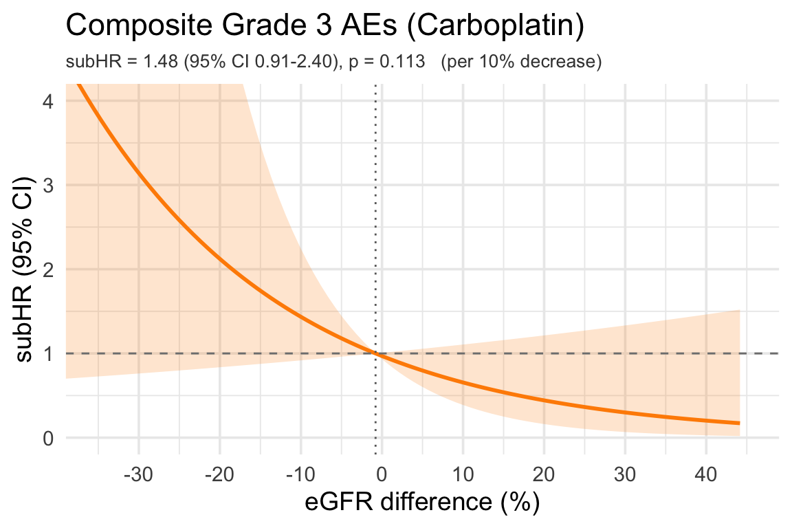
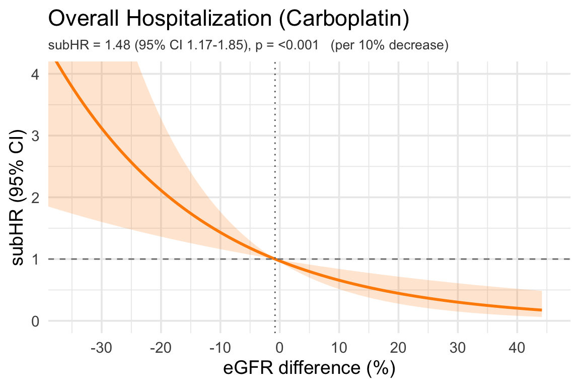
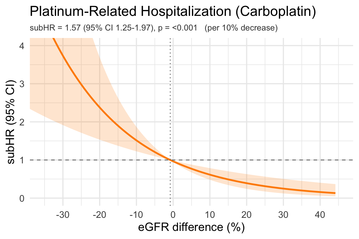
Because egfr_difference = 100 × ((eGFR − CG) / CG) = 100 × (egfr_ratio − 1), this is a pure re-centring and rescaling of the eGFR ratio: the reference point moves from 1 to 0 %. The underlying Fine-Gray fits are therefore the same models as §9 of the Sherley project’s Carboplatin Cohort page — identical p-values. The reported subHRs differ only because this page reports them per 10 % decrease in eGFR difference, whereas §9 reports per 0.1-unit increase in the ratio; the two are reciprocals of each other.

# Force UTF-8 locale so captions and other strings render real Unicode
# (e.g. em-dash) instead of <U+2014> escape sequences.
invisible(Sys.setlocale("LC_ALL", "en_US.UTF-8"))
library(tidyverse)
library(scales)
library(ggplot2)
library(tidycmprsk)
library(ggsurvfit)
library(gtsummary)
library(officer)
library(rvg)

# Output directory for downloadable PowerPoint plots (plots/grant/<name>.pptx).
pptx_dir <- normalizePath("docs/plots/grant", winslash = "/", mustWork = FALSE)
dir.create(pptx_dir, recursive = TRUE, showWarnings = FALSE)

# Save the given ggplot as an editable PowerPoint slide via rvg::dml, named by
# the calling chunk's label. Mirrors the helper in the Sherley project's
# sherley_carbo.qmd; the
# post-render script scripts/inject_pptx_links.py then injects a per-plot
# download link beneath each figure in the rendered HTML.
.save_plot_pptx <- function(p, name = NULL) {
  if (is.null(p) || !inherits(p, "ggplot")) return(invisible(NULL))
  if (is.null(name)) {
    name <- tryCatch(knitr::opts_current$get("label"), error = function(e) NULL)
  }
  if (is.null(name)) return(invisible(NULL))
  safe <- gsub("[^A-Za-z0-9]+", "_", name)
  out  <- file.path(pptx_dir, paste0(safe, ".pptx"))
  ok <- tryCatch({
    pp <- officer::read_pptx()
    pp <- officer::add_slide(pp, layout = "Title and Content", master = "Office Theme")
    pp <- officer::ph_with(
      pp,
      value = rvg::dml(ggobj = p),
      location = officer::ph_location_type(type = "body")
    )
    print(pp, target = out)
    TRUE
  }, error = function(e) FALSE)
  invisible(if (ok) paste0("plots/grant/", safe, ".pptx") else NULL)
}

# Format the exposure-effect subtitle: subHR (or HR) per `scale` units with
# 95% Wald CI and p-value, extracted from the Fine-Gray / Cox PH fit.
.hr_subtitle <- function(beta, V_beta, scale = 1,
                         hr_type = "subHR",
                         unit_label = "per 1-unit increase") {
  se   <- sqrt(V_beta)
  hr   <- exp(beta * scale)
  b1   <- exp((beta - 1.96 * se) * scale)
  b2   <- exp((beta + 1.96 * se) * scale)
  # A negative `scale` (reporting per unit DECREASE) reverses the bound order,
  # so sort rather than assuming b1 <= b2.
  lcl  <- min(b1, b2)
  ucl  <- max(b1, b2)
  pval <- 2 * (1 - pnorm(abs(beta / se)))
  p_str <- ifelse(pval < 0.001, "<0.001", sprintf("%.3f", pval))
  sprintf("%s = %.2f (95%% CI %.2f-%.2f), p = %s   (%s)",
          hr_type, hr, lcl, ucl, p_str, unit_label)
}

# Placeholder for outcomes whose design matrix is singular on this sub-cohort.
.plot_failed <- function(label = "Model could not be fit") {
  p <- ggplot() +
    annotate("text", x = 0.5, y = 0.5,
             label = paste0(label, "\n(singular design — cohort too small)"),
             size = 3.5) +
    coord_cartesian(xlim = c(0, 1), ylim = c(0, 1)) +
    theme_void()
  .save_plot_pptx(p)
  p
}

# Analysis data is produced by the Sherley project's data pipeline
# (Sherley/qmd/sherley_data.qmd writes this file). Load the whole cohort, then
# keep only carboplatin patients.
sherley_rds <- "/Users/to909/Desktop/Meg/Sherley/sherley_final_master.rds"
dat <- readRDS(sherley_rds) %>%
  filter(platin_group == "Carboplatin")

dat <- dat %>%
  mutate(
    # BSA-adjusted CKD-EPI Cr-Cys (mL/min) vs Cockcroft-Gault CrCl (mL/min).
    # Relative difference expressed as a PERCENT; 0 % = the two estimators agree.
    egfr_difference = 100 * (ckd_epi_gfr_cre_cys_unindex - cockcroft) / cockcroft,
    # Binary exposures for the adjusted CIF sections (§6, §7.3). dose_diff_pct
    # comes from the data pipeline:
    #   100 * (carbo_dose_redcap - carbo_dose_cre_cys) / carbo_dose_cre_cys
    egfr_diff_lt_neg10 = as.integer(egfr_difference < -10),
    dose_pct_ge10      = as.integer(dose_diff_pct >= 10)
  )

cat("Carboplatin cohort N =", nrow(dat), "\n")

Carboplatin cohort N = 121 

cat("eGFR difference available for N =", sum(!is.na(dat$egfr_difference)), "\n")

eGFR difference available for N = 121 

2 Carboplatin Dose Administered

Actual carboplatin dose administered (REDCap field carbo_dose_redcap, mg) across the 121-patient carboplatin cohort. All 121 have a thoracic primary and every patient has a recorded dose, so the denominator is the full cohort.

dose_vals <- dat$carbo_dose_redcap
dose_vals <- dose_vals[!is.na(dose_vals)]

tibble::tibble(
  Statistic = c("N with a recorded dose", "Mean (SD)", "Median (IQR)",
                "Range (min – max)"),
  Value = c(
    as.character(length(dose_vals)),
    sprintf("%.1f (%.1f) mg", mean(dose_vals), sd(dose_vals)),
    sprintf("%.1f (%.1f, %.1f) mg", median(dose_vals),
            quantile(dose_vals, 0.25), quantile(dose_vals, 0.75)),
    sprintf("%.1f – %.1f mg", min(dose_vals), max(dose_vals))
  )
) %>%
  knitr::kable(align = c("l", "r"),
               caption = "Actual carboplatin dose administered (mg), carboplatin cohort.")

Actual carboplatin dose administered (mg), carboplatin cohort.

Statistic	Value
N with a recorded dose	121
Mean (SD)	503.4 (124.6) mg
Median (IQR)	506.0 (407.5, 590.5) mg
Range (min – max)	197.4 – 750.0 mg

3 eGFR Difference Distribution (Carboplatin)

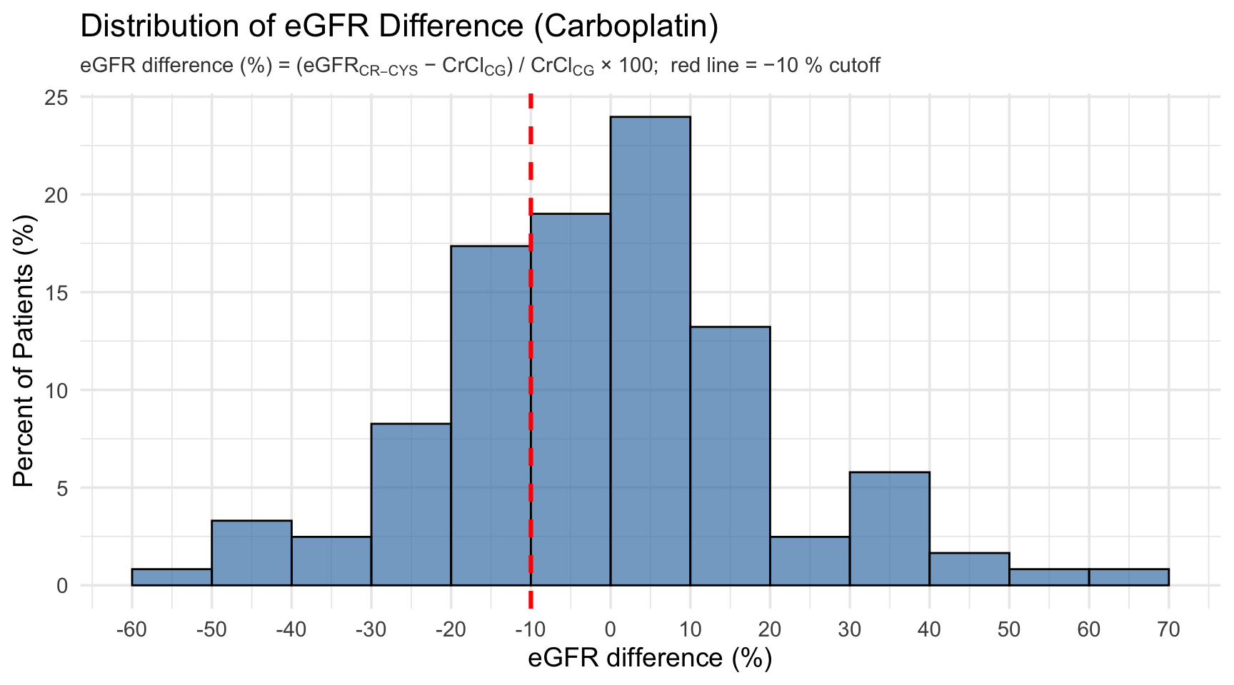
Mirrors §4 of the Sherley Carboplatin Cohort page, re-expressed as a percentage. Bins are 10 % wide with an axis tick at every bin edge. The red dashed line marks −10 % — the randomization cutoff.

diff_hist <- dat %>% filter(!is.na(egfr_difference))

ggplot(diff_hist, aes(x = egfr_difference)) +
  geom_histogram(aes(y = after_stat(count) / sum(after_stat(count)) * 100),
                 binwidth = 10, boundary = 0,
                 fill = "steelblue", color = "black", alpha = 0.7) +
  geom_vline(xintercept = -10, linetype = "dashed", color = "red",
             linewidth = 1.1) +
  labs(title = "Distribution of eGFR Difference (Carboplatin)",
       subtitle = expression(paste("eGFR difference (%) = (eGFR"[CR-CYS],
                                   " − CrCl"[CG], ") / CrCl"[CG], " × 100;  red line = −10 % cutoff")),
       x = "eGFR difference (%)",
       y = "Percent of Patients (%)") +
  scale_x_continuous(breaks = seq(-100, 200, 10)) +
  theme_minimal(base_size = 14) +
  theme(plot.subtitle = element_text(size = 11, color = "grey25")) -> p
.save_plot_pptx(p)
p

📥 Download editable PowerPoint

q <- quantile(diff_hist$egfr_difference, c(0.025, 0.25, 0.5, 0.75, 0.975),
              na.rm = TRUE)
tibble::tibble(
  Statistic = c("N", "Median", "IQR (p25, p75)", "2.5th pct", "97.5th pct",
                "% with eGFR Cr-Cys below CG (difference < 0 %)",
                "% at or below the −10 % randomization cutoff"),
  Value = c(
    as.character(nrow(diff_hist)),
    sprintf("%.1f%%", q[["50%"]]),
    sprintf("%.1f%%, %.1f%%", q[["25%"]], q[["75%"]]),
    sprintf("%.1f%%", q[["2.5%"]]),
    sprintf("%.1f%%", q[["97.5%"]]),
    sprintf("%.1f%%", 100 * mean(diff_hist$egfr_difference < 0)),
    sprintf("%.1f%% (n = %d)",
            100 * mean(diff_hist$egfr_difference <= -10),
            sum(diff_hist$egfr_difference <= -10))
  )
) %>%
  knitr::kable(align = c("l", "r"),
               caption = "eGFR difference (%) — distribution summary (carboplatin cohort).")

eGFR difference (%) — distribution summary (carboplatin cohort).

Statistic	Value
N	121
Median	-0.8%
IQR (p25, p75)	-14.3%, 9.7%
2.5th pct	-42.6%
97.5th pct	44.2%
% with eGFR Cr-Cys below CG (difference < 0 %)	51.2%
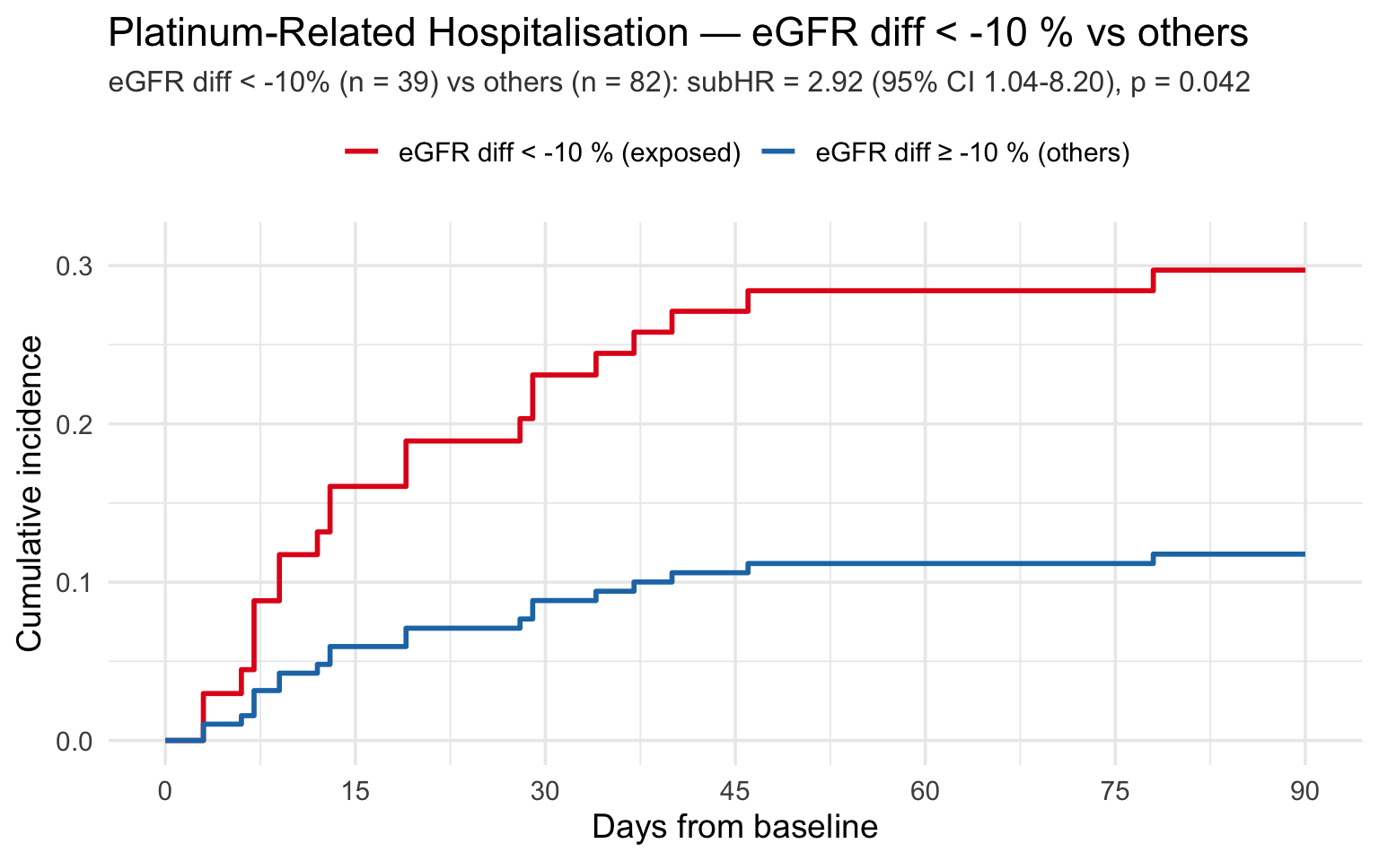
% at or below the −10 % randomization cutoff	32.2% (n = 39)

4 Predicted Dosing in the eGFR Difference ≤ −10 % Subgroup

The patients who would meet the −10 % randomization cutoff — those whose BSA-adjusted CKD-EPI Cr-Cys eGFR sits at least 10 % below their Cockcroft-Gault creatinine clearance. For this subgroup the table contrasts the carboplatin dose the Calvert formula would have produced from each kidney-function estimator against the dose actually given.

Predicted doses use Calvert at the patient’s own target AUC: dose = AUC × (min(eGFR, 125) + 25). Both arms cap the filtration estimate at 125 mL/min, so the comparison is symmetric — carbo_dose_cre_cys from the data pipeline already applies the cap (verified: it reproduces the capped formula exactly, and differs from the uncapped one by up to 53 mg), and the Cockcroft-Gault arm applies the same min(CG, 125).

The cap binds more often on the Cockcroft-Gault side in this subgroup — 11 of 39 patients exceed 125 mL/min by CG versus 3 of 39 by CKD-EPI Cr-Cys — which is expected, since the subgroup is selected for CG running high relative to Cr-Cys. The cap is therefore doing real work here: without it the Cr-Cys − CG dose gap would widen from −75.1 (41.1) mg to −113.2 (87.4) mg.

sub10 <- dat %>%
  filter(!is.na(egfr_difference), egfr_difference <= -10) %>%
  mutate(carbo_dose_cg = carbo_AUC * (pmin(cockcroft, 125) + 25))

# mean (SD) and median (IQR) for one column, formatted to 1 dp.
.msd <- function(x) {
  x <- x[!is.na(x)]
  c(sprintf("%.1f (%.1f)", mean(x), stats::sd(x)),
    sprintf("%.1f (%.1f, %.1f)", stats::median(x),
            stats::quantile(x, .25), stats::quantile(x, .75)))
}

.rows <- list(
  list("Predicted dose — CKD-EPI Cr-Cys (mg)",  sub10$carbo_dose_cre_cys),
  list("Predicted dose — Cockcroft-Gault (mg)", sub10$carbo_dose_cg),
  list("Actual dose administered (mg)",         sub10$carbo_dose_redcap),
  list("Difference — Cr-Cys − Cockcroft-Gault (mg)",
       sub10$carbo_dose_cre_cys - sub10$carbo_dose_cg),
  list("Difference — Cr-Cys − actual dose (mg)",
       sub10$carbo_dose_cre_cys - sub10$carbo_dose_redcap)
)

purrr::map_dfr(.rows, function(r) {
  v <- .msd(r[[2]])
  tibble::tibble(Measure = r[[1]], `Mean (SD)` = v[1], `Median (IQR)` = v[2])
}) %>%
  knitr::kable(
    align = c("l", "r", "r"),
    caption = sprintf(
      "Carboplatin dosing among patients with eGFR difference ≤ −10 %% (n = %d of %d carboplatin patients, %.1f %%). Negative differences mean the CKD-EPI Cr-Cys equation would have dosed lower.",
      nrow(sub10), nrow(dat), 100 * nrow(sub10) / nrow(dat)))

Carboplatin dosing among patients with eGFR difference ≤ −10 % (n = 39 of 121 carboplatin patients, 32.2 %). Negative differences mean the CKD-EPI Cr-Cys equation would have dosed lower.

Measure	Mean (SD)	Median (IQR)
Predicted dose — CKD-EPI Cr-Cys (mg)	472.0 (135.7)	476.0 (362.1, 562.7)
Predicted dose — Cockcroft-Gault (mg)	547.1 (137.1)	599.6 (427.3, 634.7)
Actual dose administered (mg)	549.8 (136.7)	600.0 (414.0, 629.5)
Difference — Cr-Cys − Cockcroft-Gault (mg)	-75.1 (41.1)	-62.1 (-96.7, -52.5)
Difference — Cr-Cys − actual dose (mg)	-77.8 (43.2)	-72.5 (-102.8, -53.0)

5 Linear subHR Curves — eGFR Difference (Carboplatin)

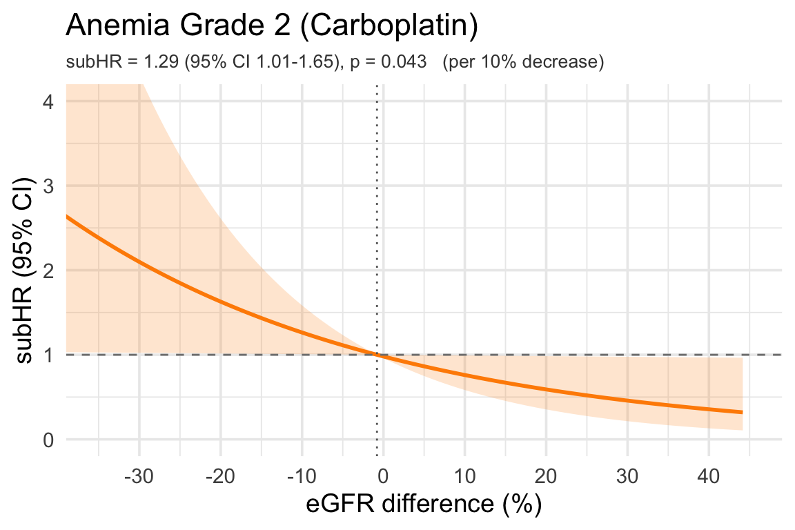
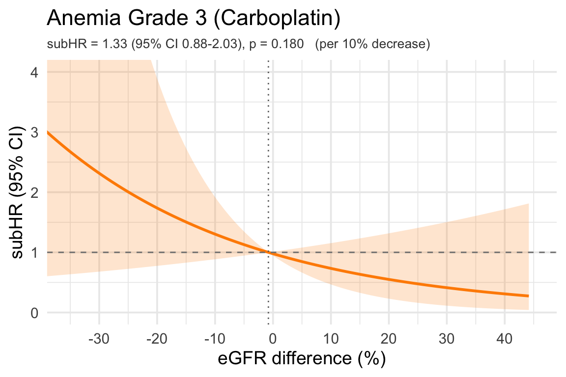
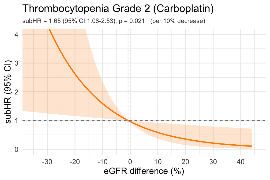
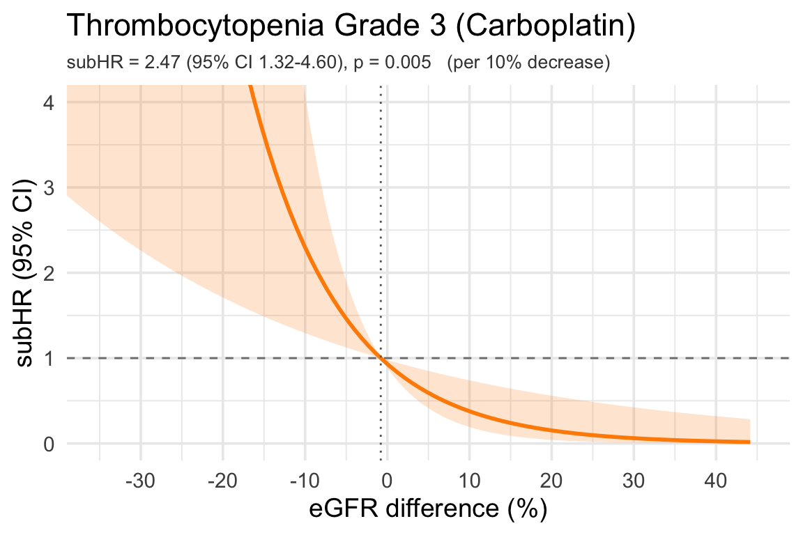
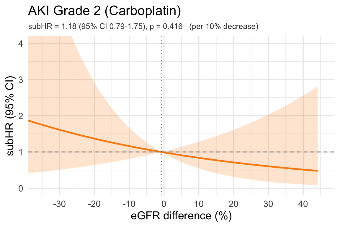
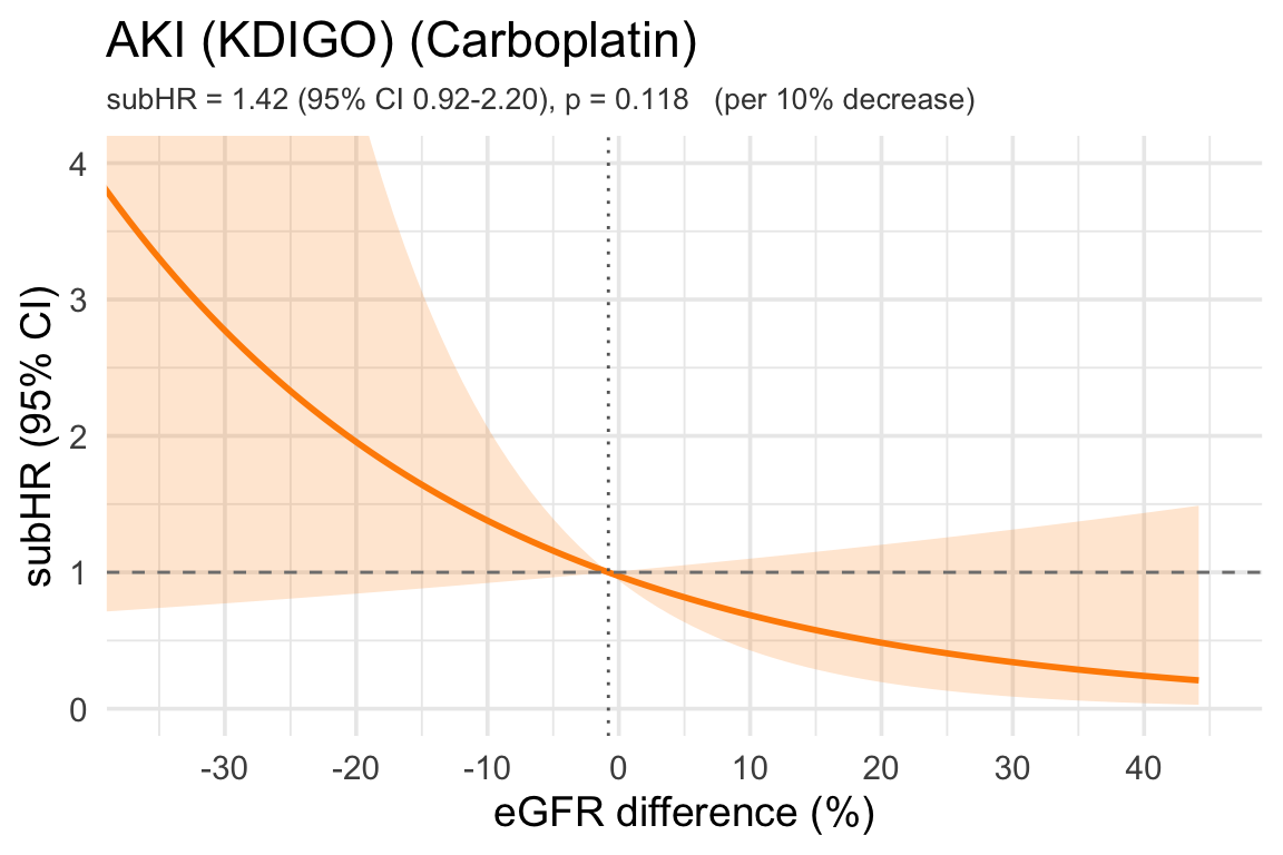
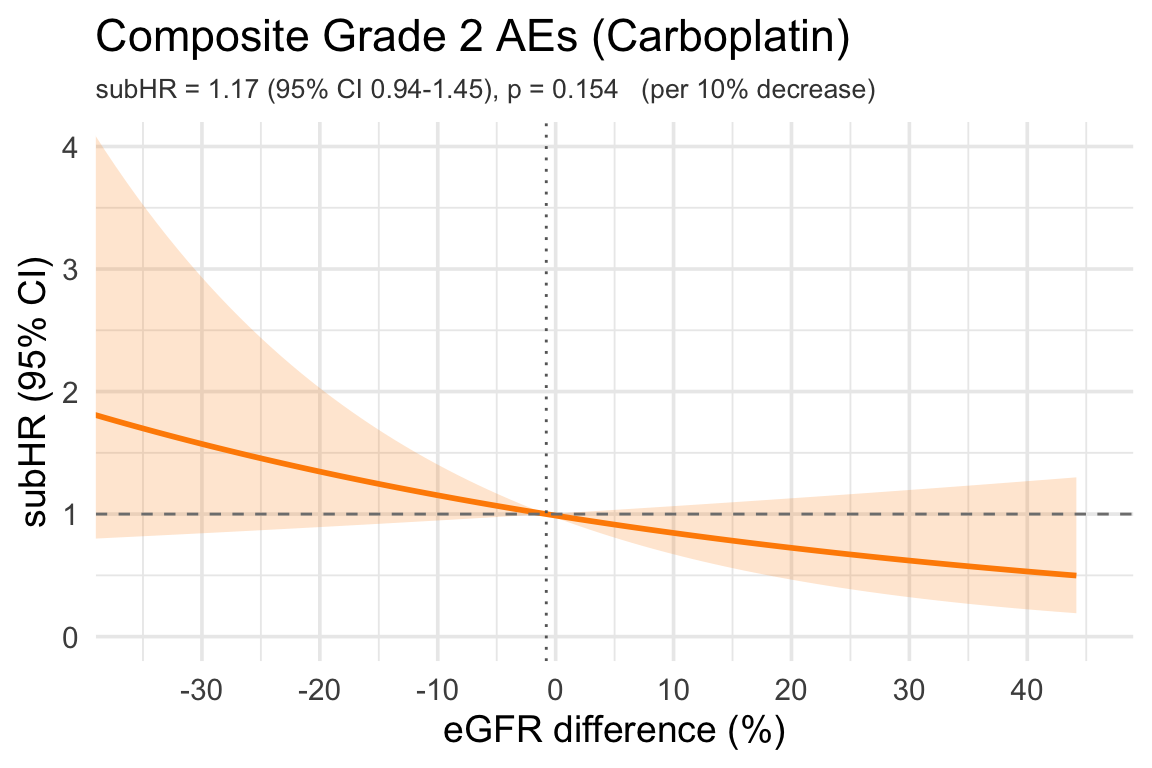
Mirrors §9.1–9.10 of the Sherley Carboplatin Cohort page, with the exposure re-expressed as the eGFR difference in percent (ticks every 10 %). Each curve is the adjusted Fine-Gray subdistribution hazard ratio as a smooth linear function of the eGFR difference, plotted relative to the cohort median (dotted vertical line). The dashed horizontal line marks subHR = 1. Reported subHRs are per 10 % decrease in eGFR difference, so a subHR above 1 means a larger CKD-EPI-Cr-Cys shortfall relative to Cockcroft-Gault carries higher risk. Models adjust for age, sex, ECOG score, ICI use and Cockcroft-Gault CrCl, plus baseline haemoglobin (anemia), baseline platelets (thrombocytopenia) or both (composite cytopenia outcomes).

# Defaults give the eGFR-difference curves of this section; §7.2 reuses the
# helper for the percent dose discrepancy via x_var / scale / labels / xlim.
plot_subhr_linear_diff <- function(time_var, status_var, extra_adj = NULL,
                                   outcome_label,
                                   x_var = "egfr_difference", scale = -10,
                                   unit_label = "per 10% decrease",
                                   x_lab = "eGFR difference (%)",
                                   xlim = c(-35, 45)) {
  base_adj <- c("age", "sex", "ecog_score", "ici", "cockcroft")
  keep <- c(x_var, time_var, status_var, base_adj, extra_adj)
  d <- dat %>% dplyr::select(all_of(keep)) %>% tidyr::drop_na()

  adj_df <- d[, c(base_adj, extra_adj), drop = FALSE]
  X_adj <- model.matrix(~ ., data = adj_df)[, -1, drop = FALSE]
  X <- cbind(d[[x_var]], X_adj)
  colnames(X)[1] <- x_var

  stat_num <- suppressWarnings(as.integer(as.character(d[[status_var]])))
  time_num <- as.numeric(d[[time_var]])

  fit <- tryCatch(
    cmprsk::crr(ftime = time_num, fstatus = stat_num,
                cov1 = X, failcode = 1),
    error = function(e) NULL
  )
  if (is.null(fit)) return(.plot_failed(outcome_label))

  beta   <- fit$coef[1]
  V_beta <- fit$var[1, 1]
  # x_var is in percentage points, so beta is per 1 pp. scale = -10 reports per
  # 10 % DECREASE, +10 per 10 % increase (sign handled in .hr_subtitle).
  subtitle_str <- .hr_subtitle(beta, V_beta, scale = scale,
                               hr_type = "subHR",
                               unit_label = unit_label)

  ref_x  <- median(d[[x_var]], na.rm = TRUE)
  grid_x <- seq(quantile(d[[x_var]], 0.025, na.rm = TRUE),
                quantile(d[[x_var]], 0.975, na.rm = TRUE),
                length.out = 100)

  log_hr <- beta * (grid_x - ref_x)
  se     <- sqrt((grid_x - ref_x)^2 * V_beta)

  df_plot <- tibble(
    x     = grid_x,
    subhr = exp(log_hr),
    lcl   = exp(log_hr - 1.96 * se),
    ucl   = exp(log_hr + 1.96 * se)
  )

  ggplot(df_plot, aes(x = x, y = subhr)) +
    geom_ribbon(aes(ymin = lcl, ymax = ucl), alpha = 0.2, fill = "darkorange") +
    geom_line(color = "darkorange", linewidth = 1) +
    geom_hline(yintercept = 1, linetype = "dashed", color = "grey50") +
    geom_vline(xintercept = ref_x, linetype = "dotted", color = "grey40") +
    labs(x = x_lab,
         y = "subHR (95% CI)",
         title = outcome_label,
         subtitle = subtitle_str) +
    scale_x_continuous(breaks = seq(-100, 100, 10)) +
    coord_cartesian(xlim = xlim, ylim = c(0, 4)) +
    theme_minimal(base_size = 14) +
    theme(plot.subtitle = element_text(size = 10, color = "grey25")) -> p
  .save_plot_pptx(p)
  p
}

5.1 Anemia Grade 2

plot_subhr_linear_diff("cmp_time_anemia_2", "cmp_status_anemia_2",
                       "pre_HGB_45days", "Anemia Grade 2 (Carboplatin)")

📥 Download editable PowerPoint

5.2 Anemia Grade 3

plot_subhr_linear_diff("cmp_time_anemia_3", "cmp_status_anemia_3",
                       "pre_HGB_45days", "Anemia Grade 3 (Carboplatin)")

📥 Download editable PowerPoint

5.3 Thrombocytopenia Grade 2

plot_subhr_linear_diff("cmp_time_throm_2", "cmp_status_throm_2",
                       "pre_PLT_45days", "Thrombocytopenia Grade 2 (Carboplatin)")

📥 Download editable PowerPoint

5.4 Thrombocytopenia Grade 3

plot_subhr_linear_diff("cmp_time_throm_3", "cmp_status_throm_3",
                       "pre_PLT_45days", "Thrombocytopenia Grade 3 (Carboplatin)")

📥 Download editable PowerPoint

5.5 AKI Grade 2

plot_subhr_linear_diff("cmp_time_aki_2", "cmp_status_aki_2",
                       NULL, "AKI Grade 2 (Carboplatin)")

📥 Download editable PowerPoint

5.6 AKI (KDIGO)

plot_subhr_linear_diff("cmp_time_aki_kdigo", "cmp_status_aki_kdigo",
                       NULL, "AKI (KDIGO) (Carboplatin)")

📥 Download editable PowerPoint

5.7 Composite Grade 2 AEs

plot_subhr_linear_diff("cmp_time_grade_2_aes", "cmp_status_grade_2_aes",
                       c("pre_HGB_45days", "pre_PLT_45days"),
                       "Composite Grade 2 AEs (Carboplatin)")

📥 Download editable PowerPoint

5.8 Composite Grade 3 AEs

plot_subhr_linear_diff("cmp_time_grade_3_aes", "cmp_status_grade_3_aes",
                       c("pre_HGB_45days", "pre_PLT_45days"),
                       "Composite Grade 3 AEs (Carboplatin)")

📥 Download editable PowerPoint

5.9 Overall Hospitalization

plot_subhr_linear_diff("cmp_time_any_hosp", "cmp_status_any_hosp",
                       NULL, "Overall Hospitalization (Carboplatin)")

📥 Download editable PowerPoint

5.10 Platinum-Related Hospitalization

plot_subhr_linear_diff("cmp_time_side_effect", "cmp_status_side_effect",
                       NULL, "Platinum-Related Hospitalization (Carboplatin)")

📥 Download editable PowerPoint

6 Adjusted CIF — eGFR Difference < −10 % vs Others (Platinum-Related Hospitalisation)

Standardized cumulative incidence function contrasting patients with egfr_difference < -10 % (red, “exposed” — the randomization group) against all other patients (blue, “reference”). Multivariable Fine-Gray model fit with the binary exposure plus this cohort’s adjuster set (age, sex, ecog_score, ici, cockcroft); Cockcroft-Gault is retained as an adjuster so the difference variable carries no residual creatinine-clearance information. Curves are adjusted (standardized) via g-computation: for every patient predict the CIF under exposure = 1 and under exposure = 0, then average the two CIF curves over the whole cohort. Y-axis is cumulative incidence of platinum-related hospitalisation, x-axis is days from baseline; death is the competing event.

# Standardized CIF for a binary (0/1) exposure column of `dat`. Defaults give
# this section's eGFR-difference contrast; §7.3 reuses it for the excess dose.
adj_cif_binary <- function(time_var, status_var, extra_pre = NULL, label,
                           expo_var = "egfr_diff_lt_neg10",
                           lab_exp  = "eGFR diff < -10 % (exposed)",
                           lab_ref  = "eGFR diff ≥ -10 % (others)",
                           sub_exp  = "eGFR diff < -10%") {
  base_adj <- c("age", "sex", "ecog_score", "ici", "cockcroft")
  d <- dat %>%
    dplyr::select(all_of(c(time_var, status_var, expo_var,
                           base_adj, extra_pre))) %>%
    tidyr::drop_na()

  fmla <- as.formula(paste("~",
            paste(c(expo_var, base_adj, extra_pre), collapse = " + ")))
  X_full <- model.matrix(fmla, data = d)[, -1, drop = FALSE]

  stat_num <- suppressWarnings(as.integer(as.character(d[[status_var]])))
  time_num <- as.numeric(d[[time_var]])

  fit <- tryCatch(
    cmprsk::crr(ftime = time_num, fstatus = stat_num,
                cov1 = X_full, failcode = 1),
    error = function(e) NULL
  )
  if (is.null(fit)) return(.plot_failed(label))

  beta_e <- unname(fit$coef[1])
  se_e   <- sqrt(fit$var[1, 1])
  hr     <- exp(beta_e)
  lcl    <- exp(beta_e - 1.96 * se_e)
  ucl    <- exp(beta_e + 1.96 * se_e)
  pval   <- 2 * (1 - pnorm(abs(beta_e / se_e)))
  p_str  <- ifelse(pval < 0.001, "<0.001", sprintf("%.3f", pval))
  n_exp  <- sum(d[[expo_var]] == 1)
  n_ref  <- sum(d[[expo_var]] == 0)
  subtitle_str <- sprintf(
    "%s (n = %d) vs others (n = %d): subHR = %.2f (95%% CI %.2f-%.2f), p = %s",
    sub_exp, n_exp, n_ref, hr, lcl, ucl, p_str
  )

  X0 <- X_full; X0[, expo_var] <- 0
  X1 <- X_full; X1[, expo_var] <- 1

  pred0 <- predict(fit, X0)
  pred1 <- predict(fit, X1)

  times <- pred0[, 1]
  cif0  <- rowMeans(pred0[, -1, drop = FALSE])
  cif1  <- rowMeans(pred1[, -1, drop = FALSE])

  # Anchor both curves at CIF = 0 on day 0 and carry the last estimate out to
  # day 90 (end of follow-up), so the steps span the full 0–90-day axis.
  t_end <- 90
  df <- bind_rows(
    tibble(time = c(0, times, t_end), cif = c(0, cif0, tail(cif0, 1)),
           group = lab_ref),
    tibble(time = c(0, times, t_end), cif = c(0, cif1, tail(cif1, 1)),
           group = lab_exp)
  )
  df$group <- factor(df$group, levels = c(lab_exp, lab_ref))

  ymax <- max(df$cif, na.rm = TRUE)

  ggplot(df, aes(x = time, y = cif, color = group)) +
    geom_step(linewidth = 1) +
    scale_color_manual(values = setNames(c("#E31A1C", "#1F78B4"),
                                         c(lab_exp, lab_ref))) +
    scale_x_continuous(breaks = seq(0, t_end, by = 15)) +
    coord_cartesian(xlim = c(0, t_end), ylim = c(0, max(0.05, ymax * 1.05))) +
    labs(x = "Days from baseline",
         y = "Cumulative incidence",
         color = NULL,
         title = label,
         subtitle = subtitle_str) +
    theme_minimal(base_size = 14) +
    theme(legend.position = "top",
          plot.subtitle = element_text(size = 12, color = "grey25")) -> p
  .save_plot_pptx(p)
  p
}

adj_cif_binary("cmp_time_side_effect", "cmp_status_side_effect",
               NULL, "Platinum-Related Hospitalisation — eGFR diff < -10 % vs others")

📥 Download editable PowerPoint

7 Dose Discrepancy (%) — Administered vs eGFR_CR-CYS-Predicted Dose

Carboplatin dose discrepancy expressed as a percent of the eGFR_CR-CYS-predicted dose:

\[ \text{Dose discrepancy (\%)} \;=\; \frac{\text{Dose}_{\text{administered}} - \text{Dose}_{\text{CR-CYS predicted}}}{\text{Dose}_{\text{CR-CYS predicted}}} \times 100 \]

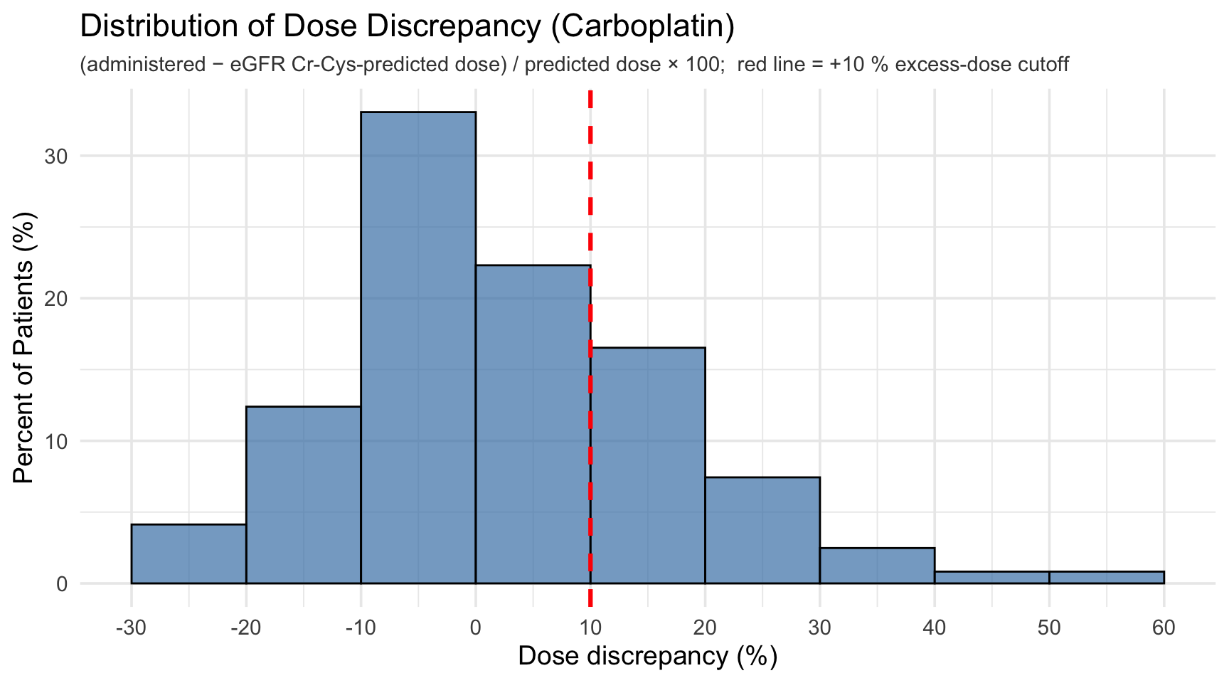
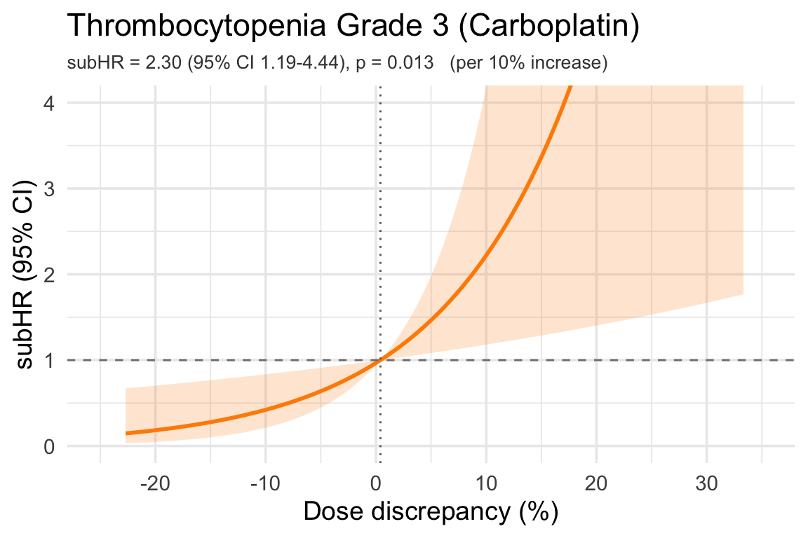
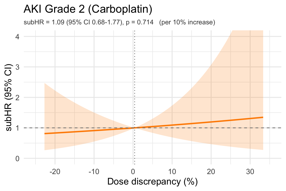
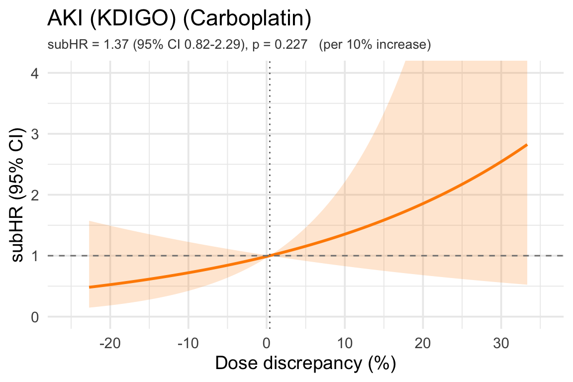
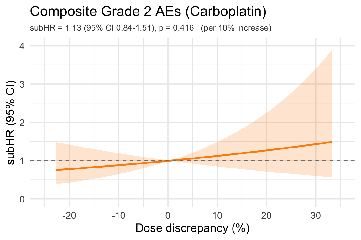
The predicted dose is the Calvert dose at the patient’s own target AUC from the BSA-adjusted CKD-EPI Cr-Cys eGFR (mL/min), capped at 125 mL/min: AUC × (min(eGFR, 125) + 25) — the same carbo_dose_cre_cys used on the Sherley Carboplatin Cohort page (pipeline variable dose_diff_pct). A positive value means the administered dose was higher than predicted, a negative value lower; for example 550 mg administered versus 500 mg predicted is a +10 % discrepancy. This is the percent analogue of the Sherley paper’s excess-dose definition (≥ 25 mg above the predicted dose): here an excess dose is one ≥ 10 % above the eGFR_CR-CYS-predicted dose.

7.1 Distribution

Bins are 10 % wide with an axis tick at every bin edge. The red dashed line marks +10 %, the excess-dose cutoff.

dose_hist <- dat %>% filter(!is.na(dose_diff_pct))

ggplot(dose_hist, aes(x = dose_diff_pct)) +
  geom_histogram(aes(y = after_stat(count) / sum(after_stat(count)) * 100),
                 binwidth = 10, boundary = 0,
                 fill = "steelblue", color = "black", alpha = 0.7) +
  geom_vline(xintercept = 10, linetype = "dashed", color = "red",
             linewidth = 1.1) +
  labs(title = "Distribution of Dose Discrepancy (Carboplatin)",
       subtitle = "(administered − eGFR Cr-Cys-predicted dose) / predicted dose × 100;  red line = +10 % excess-dose cutoff",
       x = "Dose discrepancy (%)",
       y = "Percent of Patients (%)") +
  scale_x_continuous(breaks = seq(-100, 200, 10)) +
  theme_minimal(base_size = 14) +
  theme(plot.subtitle = element_text(size = 11, color = "grey25")) -> p
.save_plot_pptx(p)
p

📥 Download editable PowerPoint

qd <- quantile(dose_hist$dose_diff_pct, c(0.025, 0.25, 0.5, 0.75, 0.975))
n_dd         <- nrow(dose_hist)
n_excess10   <- sum(dose_hist$dose_diff_pct >= 10)
pct_excess10 <- 100 * n_excess10 / n_dd
n_under10    <- sum(dose_hist$dose_diff_pct <= -10)
n_within10   <- sum(abs(dose_hist$dose_diff_pct) < 10)
n_overlap    <- sum(dose_hist$dose_diff_pct >= 10 &
                      dose_hist$egfr_difference < -10, na.rm = TRUE)
r_dd_egfr    <- cor(dose_hist$dose_diff_pct, dose_hist$egfr_difference,
                    use = "complete.obs")

tibble::tibble(
  Statistic = c("N", "Median", "IQR (p25, p75)", "2.5th pct", "97.5th pct",
                "Excess dose: ≥ 10 % above predicted",
                "≥ 10 % below predicted",
                "Within ±10 % of predicted"),
  Value = c(
    as.character(n_dd),
    sprintf("%+.1f%%", qd[["50%"]]),
    sprintf("%+.1f%%, %+.1f%%", qd[["25%"]], qd[["75%"]]),
    sprintf("%+.1f%%", qd[["2.5%"]]),
    sprintf("%+.1f%%", qd[["97.5%"]]),
    sprintf("%d (%.1f%%)", n_excess10, pct_excess10),
    sprintf("%d (%.1f%%)", n_under10, 100 * n_under10 / n_dd),
    sprintf("%d (%.1f%%)", n_within10, 100 * n_within10 / n_dd)
  )
) %>%
  knitr::kable(align = c("l", "r"),
               caption = "Dose discrepancy (%) — distribution summary (carboplatin cohort).")

Dose discrepancy (%) — distribution summary (carboplatin cohort).

Statistic	Value
N	121
Median	+0.4%
IQR (p25, p75)	-6.8%, +11.4%
2.5th pct	-22.7%
97.5th pct	+33.3%
Excess dose: ≥ 10 % above predicted	34 (28.1%)
≥ 10 % below predicted	20 (16.5%)
Within ±10 % of predicted	67 (55.4%)

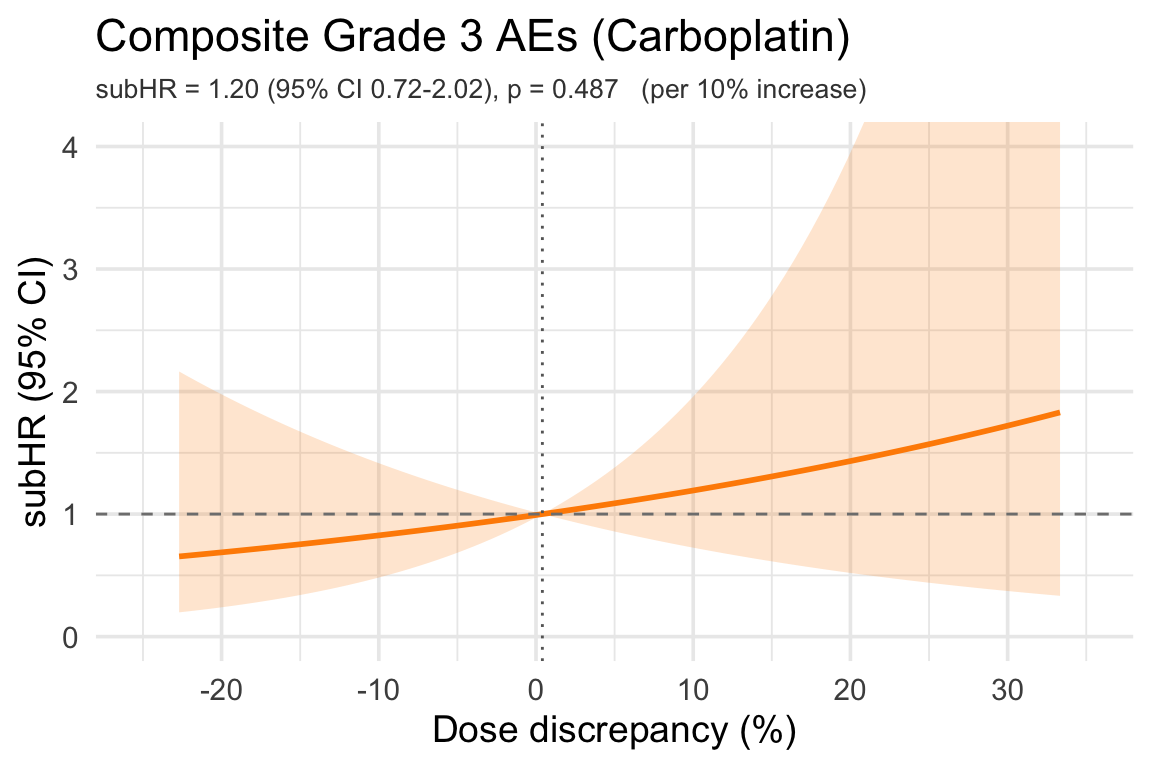
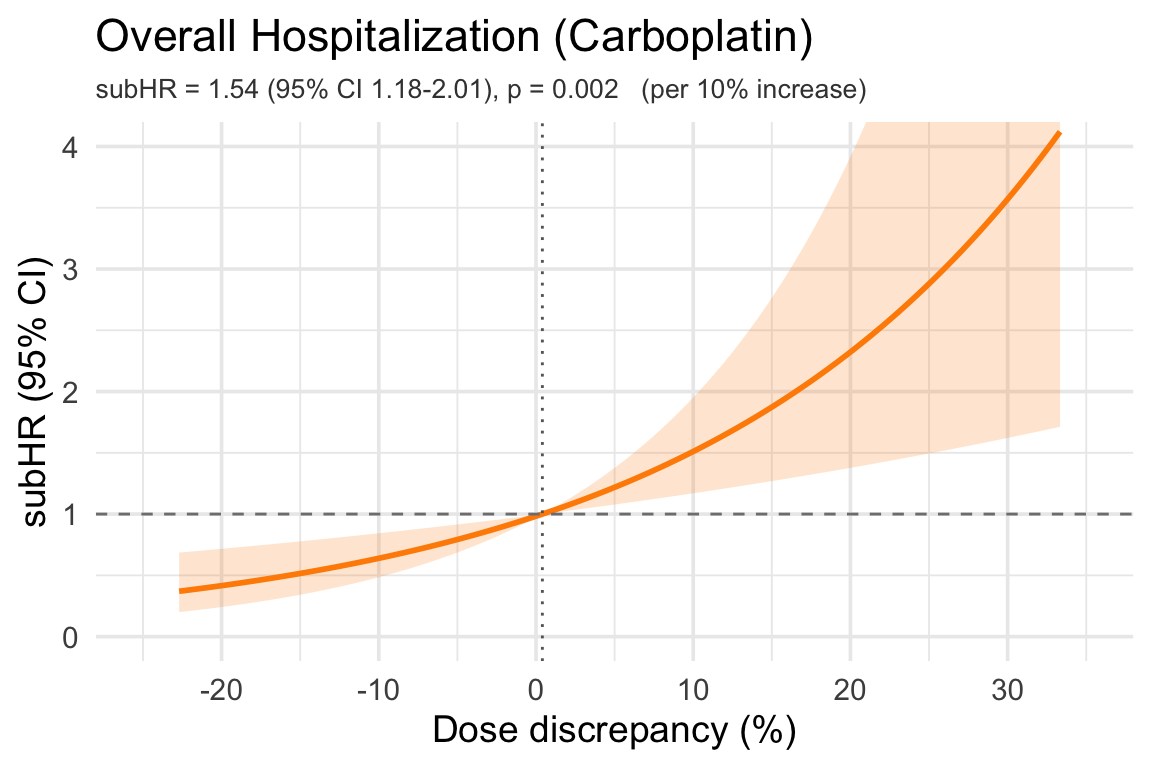
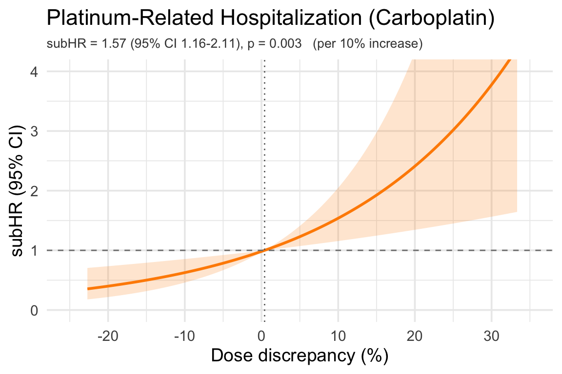
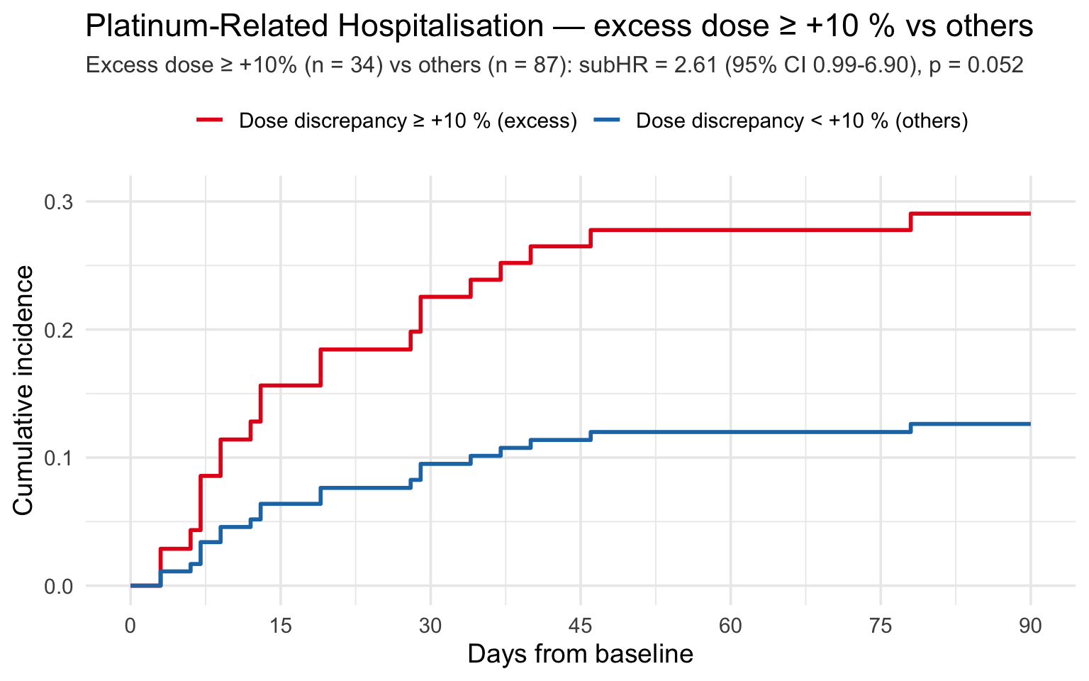
A total of 34 (28.1%) patients received an excess dose of carboplatin, defined as ≥ 10 % higher than the dose that would have been predicted using the CKD-EPI eGFR_CR-CYS equation adjusted for actual BSA. (Denominator: 121 carboplatin patients with a computable predicted dose.)

All 34 of these patients also have an eGFR difference < −10 % (§3), and the two percentages are strongly inversely correlated (r = -0.93): administered doses closely track the Cockcroft-Gault-based dose (§4), so a CKD-EPI Cr-Cys eGFR well below Cockcroft-Gault shows up as an excess dose. The excess-dose group is therefore nearly a subset of the eGFR-difference randomization group, and §7.3 largely echoes §6.

7.2 Linear subHR Curves — Dose Discrepancy (%)

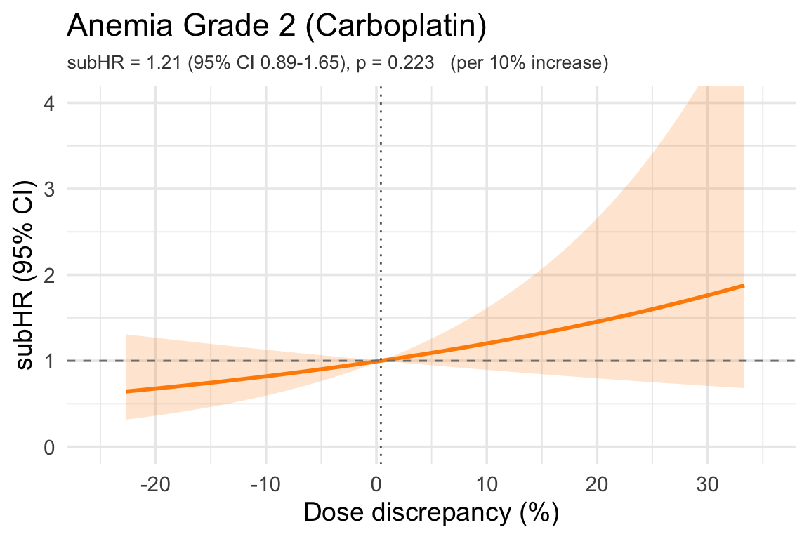
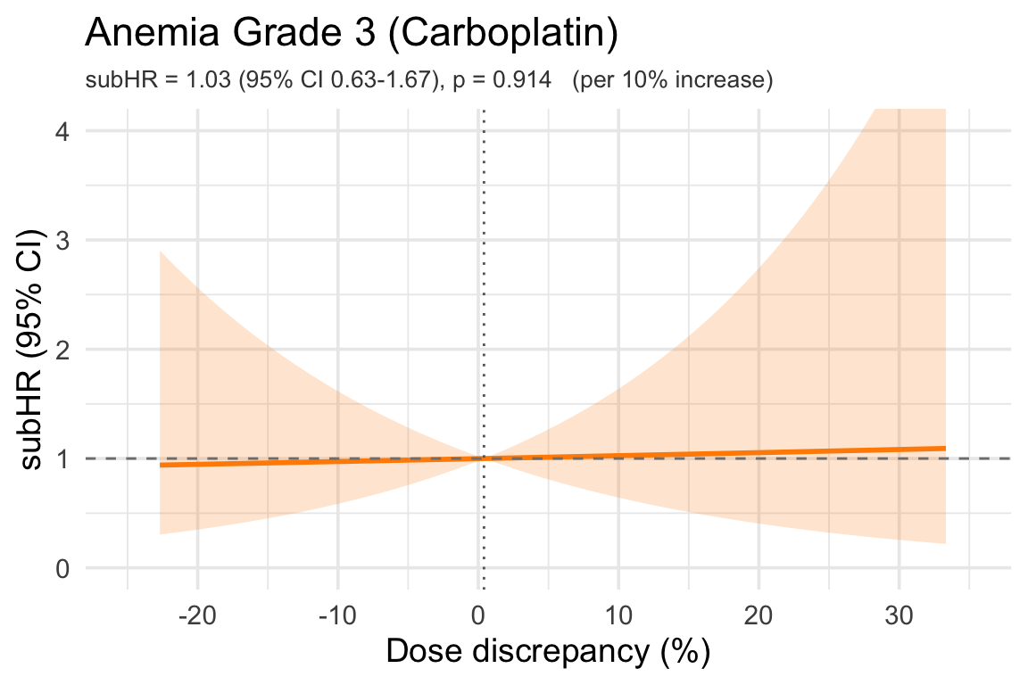
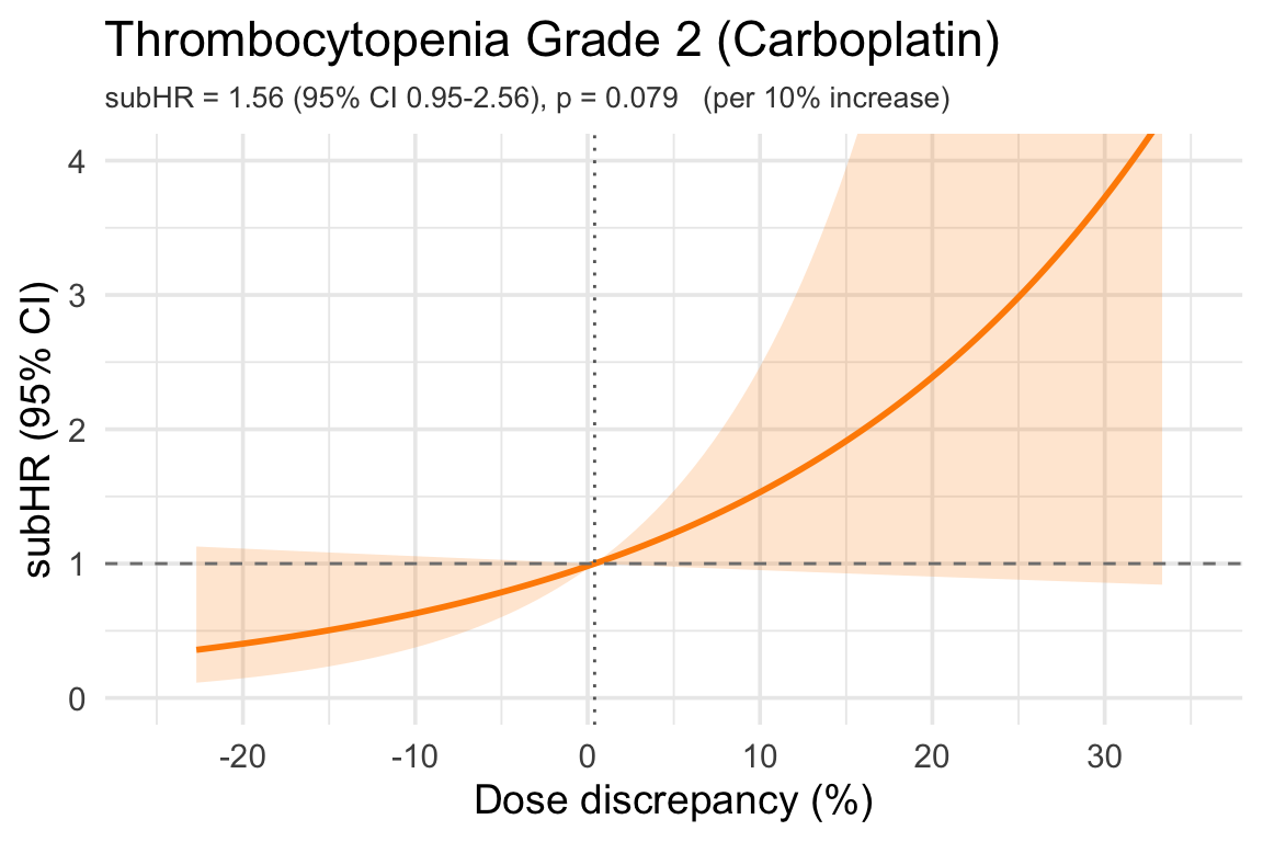
Same outcomes, adjusters and layout as §5, with the exposure being the dose discrepancy in percent. Reported subHRs are per 10 % increase in dose discrepancy (more drug given than eGFR_CR-CYS predicts), so a subHR above 1 means a larger excess dose carries higher risk. Curves are relative to the cohort median (dotted vertical line) and trimmed to the 2.5th–97.5th percentiles.

plot_subhr_dosepct <- function(time_var, status_var, extra_adj = NULL,
                               outcome_label) {
  plot_subhr_linear_diff(time_var, status_var, extra_adj, outcome_label,
                         x_var = "dose_diff_pct", scale = 10,
                         unit_label = "per 10% increase",
                         x_lab = "Dose discrepancy (%)",
                         xlim = c(-25, 35))
}

7.2.1 Anemia Grade 2

plot_subhr_dosepct("cmp_time_anemia_2", "cmp_status_anemia_2",
                   "pre_HGB_45days", "Anemia Grade 2 (Carboplatin)")

📥 Download editable PowerPoint

7.2.2 Anemia Grade 3

plot_subhr_dosepct("cmp_time_anemia_3", "cmp_status_anemia_3",
                   "pre_HGB_45days", "Anemia Grade 3 (Carboplatin)")

📥 Download editable PowerPoint

7.2.3 Thrombocytopenia Grade 2

plot_subhr_dosepct("cmp_time_throm_2", "cmp_status_throm_2",
                   "pre_PLT_45days", "Thrombocytopenia Grade 2 (Carboplatin)")

📥 Download editable PowerPoint

7.2.4 Thrombocytopenia Grade 3

plot_subhr_dosepct("cmp_time_throm_3", "cmp_status_throm_3",
                   "pre_PLT_45days", "Thrombocytopenia Grade 3 (Carboplatin)")

📥 Download editable PowerPoint

7.2.5 AKI Grade 2

plot_subhr_dosepct("cmp_time_aki_2", "cmp_status_aki_2",
                   NULL, "AKI Grade 2 (Carboplatin)")

📥 Download editable PowerPoint

7.2.6 AKI (KDIGO)

plot_subhr_dosepct("cmp_time_aki_kdigo", "cmp_status_aki_kdigo",
                   NULL, "AKI (KDIGO) (Carboplatin)")

📥 Download editable PowerPoint

7.2.7 Composite Grade 2 AEs

plot_subhr_dosepct("cmp_time_grade_2_aes", "cmp_status_grade_2_aes",
                   c("pre_HGB_45days", "pre_PLT_45days"),
                   "Composite Grade 2 AEs (Carboplatin)")

📥 Download editable PowerPoint

7.2.8 Composite Grade 3 AEs

plot_subhr_dosepct("cmp_time_grade_3_aes", "cmp_status_grade_3_aes",
                   c("pre_HGB_45days", "pre_PLT_45days"),
                   "Composite Grade 3 AEs (Carboplatin)")

📥 Download editable PowerPoint

7.2.9 Overall Hospitalization

plot_subhr_dosepct("cmp_time_any_hosp", "cmp_status_any_hosp",
                   NULL, "Overall Hospitalization (Carboplatin)")

📥 Download editable PowerPoint

7.2.10 Platinum-Related Hospitalization

plot_subhr_dosepct("cmp_time_side_effect", "cmp_status_side_effect",
                   NULL, "Platinum-Related Hospitalization (Carboplatin)")

📥 Download editable PowerPoint

7.3 Adjusted CIF — Excess Dose ≥ +10 % vs Others (Platinum-Related Hospitalisation)

Standardized cumulative incidence contrasting patients whose administered dose was ≥ 10 % above the eGFR_CR-CYS-predicted dose (red, “excess”) against all other patients (blue). Same Fine-Gray model, adjusters (age, sex, ecog_score, ici, cockcroft) and g-computation as §6; death is the competing event.

adj_cif_binary("cmp_time_side_effect", "cmp_status_side_effect",
               NULL, "Platinum-Related Hospitalisation — excess dose ≥ +10 % vs others",
               expo_var = "dose_pct_ge10",
               lab_exp  = "Dose discrepancy ≥ +10 % (excess)",
               lab_ref  = "Dose discrepancy < +10 % (others)",
               sub_exp  = "Excess dose ≥ +10%")

📥 Download editable PowerPoint

8 Downloadable PowerPoint Plots

Every figure on this page is also saved as an editable PowerPoint slide (vector graphics — text and shapes remain editable in PowerPoint). Click any link below to download the .pptx for that figure.

pptx_files <- list.files(pptx_dir, pattern = "\\.pptx$", full.names = FALSE)
if (length(pptx_files) == 0) {
  cat("*No PowerPoint files were produced during this render.*\n")
} else {
  for (f in sort(pptx_files)) {
    label <- gsub("_", " ", tools::file_path_sans_ext(f))
    cat(sprintf("- [📥 %s](plots/grant/%s)\n", label, f))
  }
}

• 📥 jx grant adjcif dosepct sideeffect
• 📥 jx grant adjcif egfrdiff sideeffect
• 📥 jx grant dosepct hist
• 📥 jx grant egfr diff hist
• 📥 jx grant linsubhr diff aki2
• 📥 jx grant linsubhr diff akikdigo
• 📥 jx grant linsubhr diff anemia2
• 📥 jx grant linsubhr diff anemia3
• 📥 jx grant linsubhr diff anyhosp
• 📥 jx grant linsubhr diff grade2
• 📥 jx grant linsubhr diff grade3
• 📥 jx grant linsubhr diff sideeffect
• 📥 jx grant linsubhr diff throm2
• 📥 jx grant linsubhr diff throm3
• 📥 jx grant linsubhr dosepct aki2
• 📥 jx grant linsubhr dosepct akikdigo
• 📥 jx grant linsubhr dosepct anemia2
• 📥 jx grant linsubhr dosepct anemia3
• 📥 jx grant linsubhr dosepct anyhosp
• 📥 jx grant linsubhr dosepct grade2
• 📥 jx grant linsubhr dosepct grade3
• 📥 jx grant linsubhr dosepct sideeffect
• 📥 jx grant linsubhr dosepct throm2
• 📥 jx grant linsubhr dosepct throm3