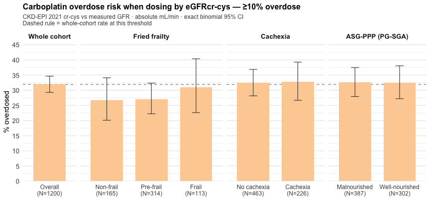
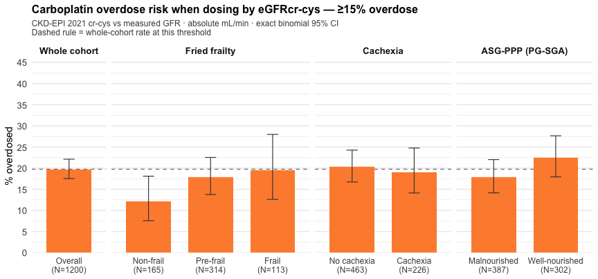
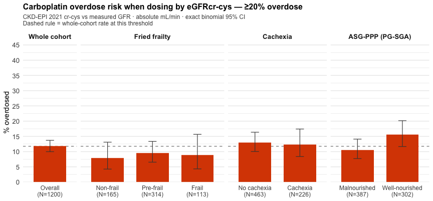
raw <- suppressWarnings(
  readxl::read_excel("/Users/to909/Desktop/Meg/Dose Leyre/Body comp data/Data/OncoGFR1200_MGH_chemo_CJASN.xlsx")
)

dat <- raw %>%
  dplyr::select(-dplyr::any_of(c("...70", "...75"))) %>%
  dplyr::mutate(
    # --- x-axis: Jiaxuan eGFR % difference ---------------------------------
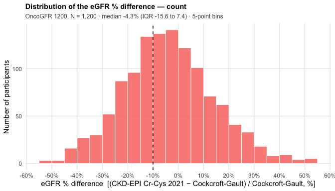
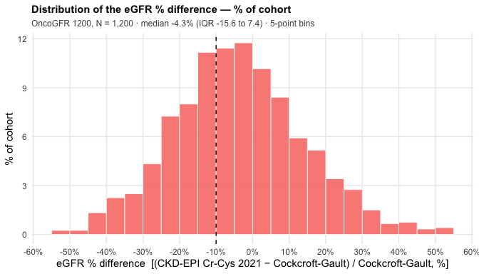
    # (eGFRcr-cys − Cockcroft-Gault) / Cockcroft-Gault × 100.
    # BOTH on the absolute mL/min scale (actual BSA, non-indexed) — the
    # `*non_index` columns. Verified: non_index = index × BSA/1.73.
    # eGFRcr-cys = CKD-EPI 2021 creatinine–cystatin C.
    egfr_pctdiff_cg = (CKDEPIcrcys21non_index - CGnon_index) / CGnon_index * 100
  )

# --- Subgroups for the frailty / cachexia figure ----------------------------
# Fried frailty class (separate file; the key is misspelled 'protocal'); 592 of
# 1200 have it. The file ships no codebook, so the 0/1/2 ordering was checked
# against external markers: mean age rises 67.4 -> 69.4 -> 70.9 (trend p = 6e-05)
# and ECOG >=2 rises 0.0% -> 5.4% -> 27.4% (p = 2e-27). Both confirm the standard
# Fried ordering, so 0 = non-frail, 1 = pre-frail, 2 = frail.
.fr <- suppressWarnings(readxl::read_excel("/Users/to909/Desktop/Meg/Dose Leyre/Body comp data/Data/Frailty data to MGH.xlsx"))
dat$fried_grp <- factor(.fr$fried_classification[match(dat$protocol, .fr$protocal)],
                        levels = c(0, 1, 2),
                        labels = c("Non-frail", "Pre-frail", "Frail"))

# Nutrition markers (separate file; key = 'Protocol Number'); 689 of 1200.
# Cachexia 0 = No, 1 = Yes. ASG-PPP / PG-SGA global rating coded 1/2.
.nut <- suppressWarnings(readxl::read_excel("/Users/to909/Desktop/Meg/Dose Leyre/Body comp data/Data/Nutrition data.xlsx"))
names(.nut) <- trimws(names(.nut))
.nk <- match(dat$protocol, .nut$`Protocol Number`)
dat$cachexia_grp <- factor(.nut$Cachexia[.nk], levels = c(0, 1),
                           labels = c("No cachexia", "Cachexia"))
# ASG-PPP direction also established from the data, and it is the OPPOSITE of the
# intuitive "higher number = worse" reading: rating 1 is the malnourished group.
# 49.6% of rating 1 are cachectic vs 11.3% of rating 2 (Fisher p = 2e-28), with
# worse ECOG (6.2% vs 3.6% at >=2) and slightly lower BMI. Labels say so, so the
# figure cannot be misread.
dat$asgppp_grp   <- factor(.nut$`ASG-PPP`[.nk], levels = c(1, 2),
                           labels = c("Malnourished", "Well-nourished"))

# --- Equation registry: the 8 dosing equations, same as the heatmap page ----
# Reference = measured GFR. The creatinine CKD-EPI column is the 2021 (race-free)
# equation; the hyphen in "EKFCcrcysnon-index" is intentional.
reg <- tibble::tribble(
  ~equation,       ~type,        ~label,             ~index_col,           ~nonindex_col,
  "CKDEPIcr21",    "eGFRcr",     "CKD-EPI 2021",     "CKDEPIcr21index",    "CKDEPIcr21non_index",
  "EKFCcr",        "eGFRcr",     "EKFC 2021",        "EKFCcrindex",        "EKFCcrnon_index",
  "CKDEPIcys",     "eGFRcys",    "CKD-EPI 2012",     "CKDEPIcysindex",     "CKDEPIcysnon_index",
  "EKFCcys",       "eGFRcys",    "EKFC 2023",        "EKFCcysindex",       "EKFCcysnon_index",
  "CKDEPIcrcys21", "eGFRcr-cys", "CKD-EPI 2021",     "CKDEPIcrcys21index", "CKDEPIcrcys21non_index",
  "EKFCcrcys",     "eGFRcr-cys", "EKFC 2023",        "EKFCcrcysindex",     "EKFCcrcysnon-index",
  "CG",            "ClCr",       "Cockcroft-Gault",  "CGindex",            "CGnon_index",
  "CKDEPI4mark",   "Panel",      "CKD-EPI 4-marker", "CKDEPI4mark",        "CKDEPI4marknon_index"
)
MGFR <- c(index = "mGFRindex", nonindex = "mGFRnon_index")

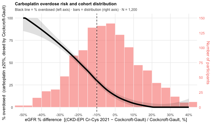
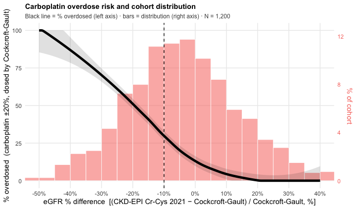
# Carboplatin Calvert (AUC 5), ±20 % band:
#   over  if 5*(eGFR+25) > 6*(mGFR+25)
#   under if 5*(eGFR+25) < 4*(mGFR+25)
carbo_class <- function(gfr, mgfr, k_hi = 6, k_lo = 4) {
  pred <- 5 * (gfr + 25)
  dplyr::case_when(is.na(gfr) | is.na(mgfr) ~ NA_character_,
                   pred > k_hi * (mgfr + 25) ~ "Overdose",
                   pred < k_lo * (mgfr + 25) ~ "Underdose", TRUE ~ "Concordant")
}

# Patient × equation table carrying the discordance index, for one GFR scale.
build_carbo_long <- function(scale = c("nonindex", "index"), data = dat) {
  scale  <- match.arg(scale)
  mgfr   <- data[[MGFR[[scale]]]]
  col_of <- function(eq) {
    r <- reg[reg$equation == eq, ]
    if (scale == "index") r$index_col[[1]] else r$nonindex_col[[1]]
  }
  purrr::map_dfr(reg$equation, function(eq) {
    tibble::tibble(
      equation        = eq,
      egfr_pctdiff_cg = data$egfr_pctdiff_cg,
      cls             = carbo_class(data[[col_of(eq)]], mgfr)
    )
  })
}
carbo_nonindex <- build_carbo_long("nonindex")
carbo_index    <- build_carbo_long("index")

# X-axis label and window. The index runs ~ -52 % to +53 % in this cohort;
# [-50, 40] holds 98.2 % of patients and keeps the smooth off sparse tails.
PCTD_CG_XLAB <- "eGFR % difference  [(CKD-EPI Cr-Cys 2021 − Cockcroft-Gault) / Cockcroft-Gault, %]"
PCTD_CG_XLIM <- c(-50, 40)
# Ticks every 10 percentage points. The set spans the full data range (-52 to
# +53) so the unclipped distribution plots are ticked end to end; Figures 1 and 3
# are clipped to PCTD_CG_XLIM, which simply drops the breaks outside it.
PCTD_CG_BREAKS <- seq(-60, 60, 10)
# The single reference marker on every panel: a black dashed line at -10 %.
REF_LINE <- -10

# Shared x-axis scale + tick styling, so every figure on this page lines up.
pctd_x <- function() {
  list(
    ggplot2::scale_x_continuous(
      breaks = PCTD_CG_BREAKS,
      labels = paste0(PCTD_CG_BREAKS, "%"),
      minor_breaks = NULL),
    ggplot2::theme(
      axis.ticks.x        = ggplot2::element_line(colour = "black", linewidth = 0.4),
      axis.ticks.length.x = grid::unit(4, "pt"),
      panel.grid.minor.x  = ggplot2::element_blank()))
}
ref_vline <- function() {
  ggplot2::geom_vline(xintercept = REF_LINE, linetype = "dashed",
                      colour = "black", linewidth = 0.5)
}

# Carboplatin red — the same hue as the "Carboplatin (±20%)" line in the 5-drug panels.
CARBO_RED <- "#F8766D"

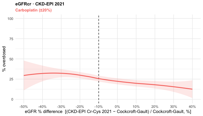
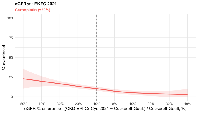
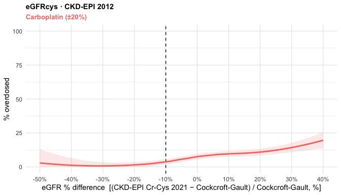
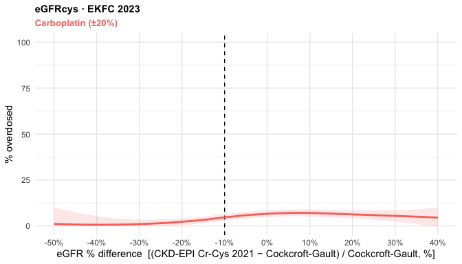
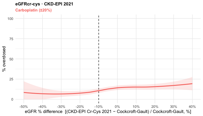
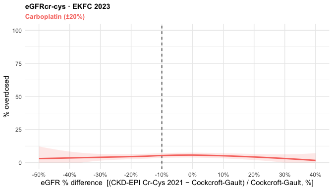
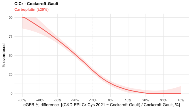
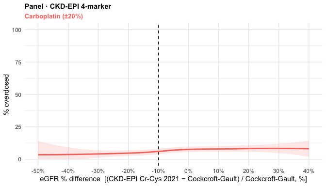
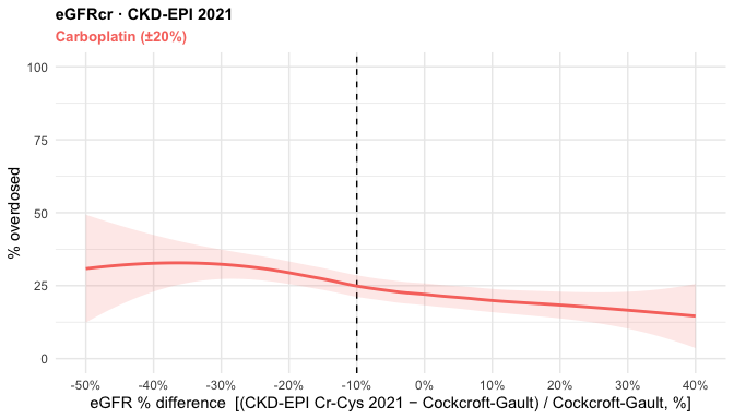
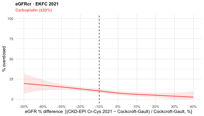
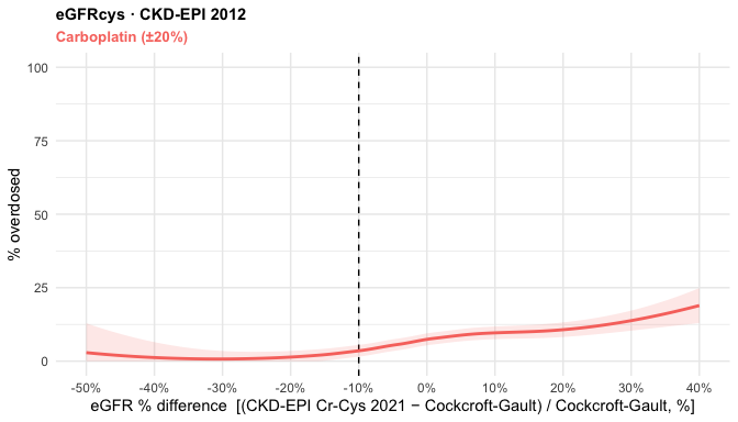
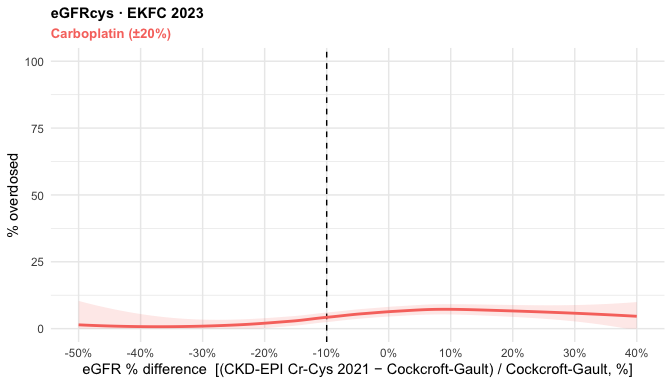
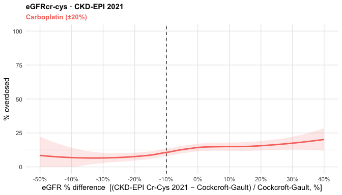
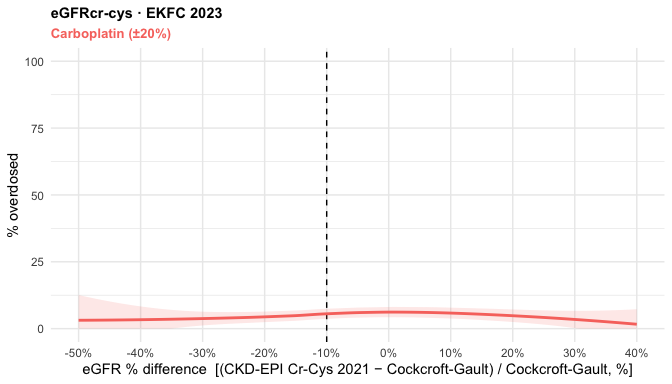
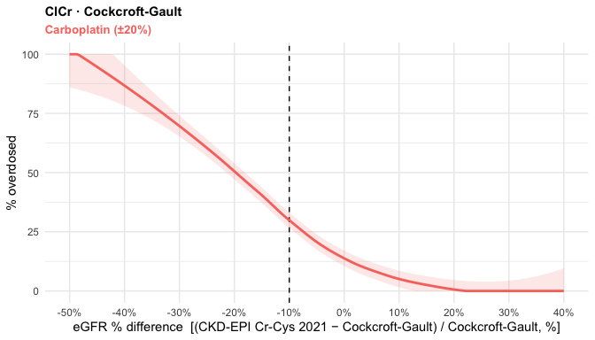
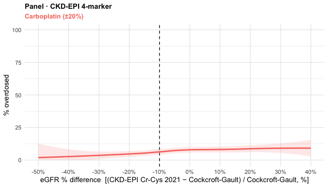
# One panel per equation: a single LOESS smooth of P(overdose) for carboplatin
# ±20 %, as a function of the discordance index. Binary 0/1 → % via the smooth.
grant_loess <- function(cl, eq, direction = "Overdose") {
  r   <- reg[reg$equation == eq, ]
  ttl <- paste0(r$type, " · ", r$label)
  d <- cl %>%
    dplyr::filter(equation == eq, !is.na(cls), !is.na(egfr_pctdiff_cg)) %>%
    dplyr::mutate(y = as.integer(cls == direction) * 100)

  # Fit the LOESS explicitly rather than letting geom_smooth do it, so the drawn
  # curve and its band can be clamped to [0, 100]. An unconstrained smooth of a
  # 0/1 outcome overshoots at the sparse ends (the Cockcroft-Gault panel reaches
  # ~105 % on the left), which would be indefensible in a grant figure. The fit
  # itself is untouched — only what is drawn is clipped to the possible range.
  fit  <- stats::loess(y ~ x, span = 0.9,
                       data = data.frame(x = d$egfr_pctdiff_cg, y = d$y))
  gx   <- seq(PCTD_CG_XLIM[1], PCTD_CG_XLIM[2], length.out = 200)
  pr   <- stats::predict(fit, newdata = data.frame(x = gx), se = TRUE)
  clip <- function(v) pmin(pmax(v, 0), 100)
  band <- data.frame(x   = gx,
                     fit = clip(pr$fit),
                     lo  = clip(pr$fit - 1.96 * pr$se.fit),
                     hi  = clip(pr$fit + 1.96 * pr$se.fit))

  ggplot2::ggplot(band, ggplot2::aes(x)) +
    ref_vline() +
    ggplot2::geom_ribbon(ggplot2::aes(ymin = lo, ymax = hi),
                         fill = CARBO_RED, alpha = 0.15) +
    ggplot2::geom_line(ggplot2::aes(y = fit), colour = CARBO_RED, linewidth = 1.0) +
    pctd_x() +
    ggplot2::coord_cartesian(xlim = PCTD_CG_XLIM, ylim = c(0, 100)) +
    ggplot2::labs(x = PCTD_CG_XLAB, y = paste0("% ", tolower(direction), "d"),
                  title = ttl,
                  subtitle = "Carboplatin (±20%)") +
    ggplot2::theme_minimal(base_size = 11) +
    ggplot2::theme(
      plot.title    = ggplot2::element_text(face = "bold", size = 11),
      plot.subtitle = ggplot2::element_text(colour = CARBO_RED, face = "bold", size = 10))
}